This article mainly introduces the detailed explanation of python programming to calculate definite integrals through the Monte Carlo method. It has certain reference value and friends in need can refer to it.
I think back then, when I was taking the postgraduate entrance examination, I wish I had known that there was such a good thing, calculating definite points. . . Just kidding, calculating definite integrals was not that simple at that time. But it did open up an idea for me to use programming languages to solve more complex mathematical problems. Let’s get to the point.
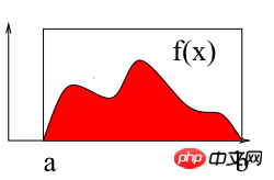
As shown in the figure above, calculating the integral of f(x) on the interval [a b] is to find the area of the red area surrounded by the curve and the X-axis. The following uses the Monte Carlo method to calculate the definite integral on the interval [2 3]: ∫(x2 4*x*sin(x))dx
# -*- coding: utf-8 -*-
import numpy as np
import matplotlib.pyplot as plt

def f(x):
  return x**2 + 4*x*np.sin(x)
def intf(x):
  return x**3/3.0+4.0*np.sin(x) - 4.0*x*np.cos(x)
a = 2;
b = 3;
# use N draws
N= 10000
X = np.random.uniform(low=a, high=b, size=N) # N values uniformly drawn from a to b
Y =f(X)  # CALCULATE THE f(x)
# 蒙特卡洛法计算定积分:面积=宽度*平均高度
Imc= (b-a) * np.sum(Y)/ N;
exactval=intf(b)-intf(a)
print "Monte Carlo estimation=",Imc, "Exact number=", intf(b)-intf(a)
# --How does the accuracy depends on the number of points(samples)? Lets try the same 1-D integral
# The Monte Carlo methods yield approximate answers whose accuracy depends on the number of draws.
Imc=np.zeros(1000)
Na = np.linspace(0,1000,1000)
exactval= intf(b)-intf(a)
for N in np.arange(0,1000):
  X = np.random.uniform(low=a, high=b, size=N) # N values uniformly drawn from a to b
  Y =f(X)  # CALCULATE THE f(x)
  Imc[N]= (b-a) * np.sum(Y)/ N;
plt.plot(Na[10:],np.sqrt((Imc[10:]-exactval)**2), alpha=0.7)
plt.plot(Na[10:], 1/np.sqrt(Na[10:]), 'r')
plt.xlabel("N")
plt.ylabel("sqrt((Imc-ExactValue)$^2$)")
plt.show()
Copy after login
##>>>
Monte Carlo estimation= 11.8181144118 Exact number= 11.8113589251
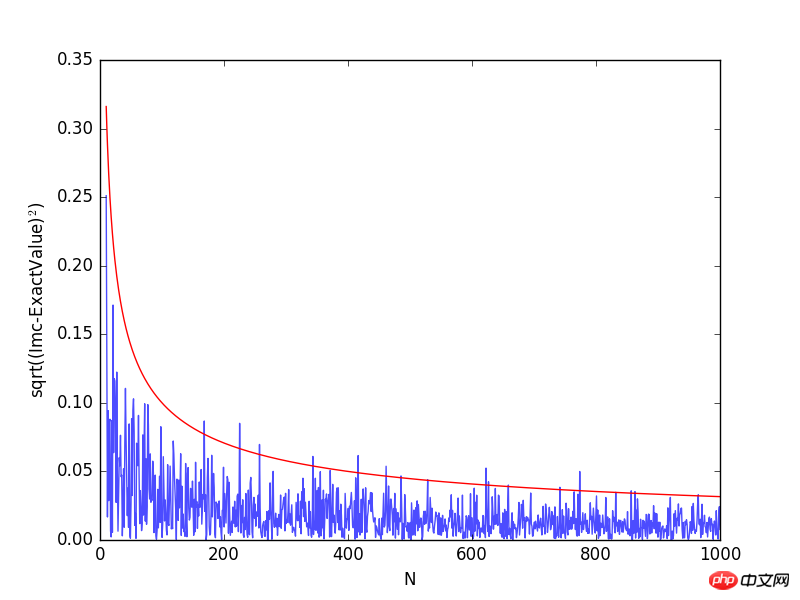
From the picture above It can be seen that as the number of sampling points increases, the calculation error gradually decreases. There are two ways to improve the accuracy of simulation results: one is to increase the number of tests N; the other is to reduce the variance σ2. Increasing the number of tests will inevitably increase the total computer time used to solve the problem. In order to improve the accuracy, The purpose is obviously inappropriate. Next, we will introduce the important sampling method to reduce the variance and improve the accuracy of the integral calculation.
The characteristic of the importance sampling method is that it does not sample from the probability distribution of a given process, but samples from a modified probability distribution, so that events that are important to the simulation results appear more often, thereby improving Sampling efficiency, reducing computational time spent on events that are insignificant to simulation results. For example, find the integral of g(x) on the interval [a b]. If uniform sampling is used, the number of sampling points generated in the interval where the function value g(x) is relatively small is the same as the number of sampling points generated in the interval where the function value is large. Close, obviously the sampling efficiency is not high. You can change the sampling probability density function to f(x), so that the shapes of f(x) and g(x) are similar, which can ensure the chance of sampling values that contribute greatly to the integral calculation to appear. is greater than the sampling value with a small contribution, that is, the integral operation can be rewritten as:

x is a random variable obtained by sampling according to the probability density f(x), obviously in the interval [a b ] should contain:

# Therefore, the integral value I can be easily regarded as the expectation of the random variable Y = g(x)/f(x), in the formula xi is a sampling point that obeys the probability density f(x)

The following example uses a normal distribution function f(x) to approximate g(x)=sin(x )*x, and select the sampling value according to the normal distribution to calculate the integral number ∫g(x)dx
# -*- coding: utf-8 -*-
# Example: Calculate ∫sin(x)xdx
# The function has a shape that is similar to Gaussian and therefore
# we choose here a Gaussian as importance sampling distribution.
from scipy import stats
from scipy.stats import norm
import numpy as np
import matplotlib.pyplot as plt
mu = 2;
sig =.7;
f = lambda x: np.sin(x)*x
infun = lambda x: np.sin(x)-x*np.cos(x)
p = lambda x: (1/np.sqrt(2*np.pi*sig**2))*np.exp(-(x-mu)**2/(2.0*sig**2))
normfun = lambda x: norm.cdf(x-mu, scale=sig)
plt.figure(figsize=(18,8)) # set the figure size
# range of integration
xmax =np.pi
xmin =0
# Number of draws
N =1000
# Just want to plot the function
x=np.linspace(xmin, xmax, 1000)
plt.subplot(1,2,1)
plt.plot(x, f(x), 'b', label=u'Original $x\sin(x)$')
plt.plot(x, p(x), 'r', label=u'Importance Sampling Function: Normal')
plt.xlabel('x')
plt.legend()
# =============================================
# EXACT SOLUTION
# =============================================
Iexact = infun(xmax)-infun(xmin)
print Iexact
# ============================================
# VANILLA MONTE CARLO
# ============================================
Ivmc = np.zeros(1000)
for k in np.arange(0,1000):
x = np.random.uniform(low=xmin, high=xmax, size=N)
Ivmc[k] = (xmax-xmin)*np.mean(f(x))
# ============================================
# IMPORTANCE SAMPLING
# ============================================
# CHOOSE Gaussian so it similar to the original functions
# Importance sampling: choose the random points so that
# more points are chosen around the peak, less where the integrand is small.
Iis = np.zeros(1000)
for k in np.arange(0,1000):
# DRAW FROM THE GAUSSIAN: xis~N(mu,sig^2)
xis = mu + sig*np.random.randn(N,1);
xis = xis[ (xis<xmax) & (xis>xmin)] ;
# normalization for gaussian from 0..pi
normal = normfun(np.pi)-normfun(0) # 注意:概率密度函数在采样区间[0 pi]上的积分需要等于1
Iis[k] =np.mean(f(xis)/p(xis))*normal # 因此,此处需要乘一个系数即p(x)在[0 pi]上的积分
plt.subplot(1,2,2)
plt.hist(Iis,30, histtype='step', label=u'Importance Sampling');
plt.hist(Ivmc, 30, color='r',histtype='step', label=u'Vanilla MC');
plt.vlines(np.pi, 0, 100, color='g', linestyle='dashed')
plt.legend()
plt.show()
Copy after login
on the interval [0 pi]
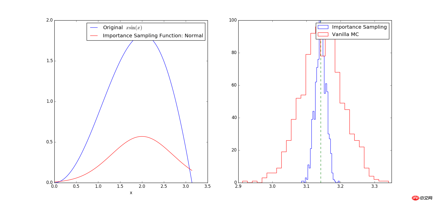
It can be seen from the figure that the shape of the curve sin(x)*x is similar to the shape of the normal distribution curve, so the number of sampling points at the peak of the curve will be greater than the position on the curve There are more low places. The result of the precise calculation is pi. As can be seen from the right picture above: both methods calculate the definite integral 1000 times. The results close to the precise value pi=3.1415 are the most. The farther away from the precise value, the smaller the number. Obviously, this is consistent with conventional. However, the difference in the square of the integral value calculated using the traditional method (red histogram) is significantly larger than that using the important sampling method (blue histogram). Therefore, using the importance sampling method to calculate can reduce the variance and improve the accuracy. In addition, it should be noted that the choice of function f(x) will affect the accuracy of the calculation results. When the function f(x) we choose is very different from g(x), the variance of the calculation results will also increase. .
Related recommendations:
How to use NotImplementedError in Python programming_python
The above is the detailed content of Detailed explanation of python programming to calculate definite integrals through Monte Carlo method. For more information, please follow other related articles on the PHP Chinese website!


![[Web front-end] Node.js quick start](https://img.php.cn/upload/course/000/000/067/662b5d34ba7c0227.png)


