

Die vier Methoden zum Eliminieren abnormaler Daten sind: 1. „Isolationswald“; 2. „Lokaler Ausreißerfaktor“;

Die Betriebsumgebung dieses Tutorials: Windows 7-System, Dell G3-Computer.
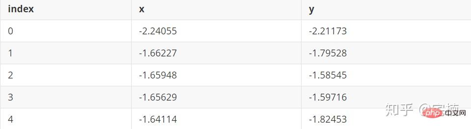
Datei test.pkl
Isolationswaldprinzip
Durch zufälliges Teilen von Features erstellen eine zufällige Gesamtstruktur und betrachten Punkte, die nach einer kleinen Anzahl von Teilungen geteilt werden können, als abnormale Punkte.
# 参考https://blog.csdn.net/ye1215172385/article/details/79762317
# 官方例子https://scikit-learn.org/stable/auto_examples/ensemble/plot_isolation_forest.html#sphx-glr-auto-examples-ensemble-plot-isolation-forest-py
import numpy as np
import matplotlib.pyplot as plt
from sklearn.ensemble import IsolationForest

rng = np.random.RandomState(42)

# 构造训练样本
n_samples = 200  #样本总数
outliers_fraction = 0.25  #异常样本比例
n_inliers = int((1. - outliers_fraction) * n_samples)
n_outliers = int(outliers_fraction * n_samples)

X = 0.3 * rng.randn(n_inliers // 2, 2)
X_train = np.r_[X + 2, X - 2]   #正常样本
X_train = np.r_[X_train, np.random.uniform(low=-6, high=6, size=(n_outliers, 2))]  #正常样本加上异常样本

# 构造模型并拟合
clf = IsolationForest(max_samples=n_samples, random_state=rng, contamination=outliers_fraction)
clf.fit(X_train)
# 计算得分并设置阈值
scores_pred = clf.decision_function(X_train)
threshold = np.percentile(scores_pred, 100 * outliers_fraction)  #根据训练样本中异常样本比例,得到阈值,用于绘图

# plot the line, the samples, and the nearest vectors to the plane
xx, yy = np.meshgrid(np.linspace(-7, 7, 50), np.linspace(-7, 7, 50))
Z = clf.decision_function(np.c_[xx.ravel(), yy.ravel()])
Z = Z.reshape(xx.shape)

plt.title("IsolationForest")
# plt.contourf(xx, yy, Z, cmap=plt.cm.Blues_r)
plt.contourf(xx, yy, Z, levels=np.linspace(Z.min(), threshold, 7), cmap=plt.cm.Blues_r)  #绘制异常点区域,值从最小的到阈值的那部分
a = plt.contour(xx, yy, Z, levels=[threshold], linewidths=2, colors='red')  #绘制异常点区域和正常点区域的边界
plt.contourf(xx, yy, Z, levels=[threshold, Z.max()], colors='palevioletred')  #绘制正常点区域,值从阈值到最大的那部分

b = plt.scatter(X_train[:-n_outliers, 0], X_train[:-n_outliers, 1], c='white',
                    s=20, edgecolor='k')
c = plt.scatter(X_train[-n_outliers:, 0], X_train[-n_outliers:, 1], c='black',
                    s=20, edgecolor='k')
plt.axis('tight')
plt.xlim((-7, 7))
plt.ylim((-7, 7))
plt.legend([a.collections[0], b, c],
           ['learned decision function', 'true inliers', 'true outliers'],
           loc="upper left")
plt.show()Hier gibt es keine Standardisierung. Sie können zuerst standardisieren und dann Ausreißer basierend auf der Standardisierung entfernen.
import numpy as np
import matplotlib.pyplot as plt
from sklearn.ensemble import IsolationForest
from scipy import stats

rng = np.random.RandomState(42)


X_train =  X_train_demo.values
outliers_fraction = 0.1
n_samples = 500
# 构造模型并拟合
clf = IsolationForest(max_samples=n_samples, random_state=rng, contamination=outliers_fraction)
clf.fit(X_train)
# 计算得分并设置阈值
scores_pred = clf.decision_function(X_train)
threshold = stats.scoreatpercentile(scores_pred, 100 * outliers_fraction)  #根据训练样本中异常样本比例,得到阈值,用于绘图

# plot the line, the samples, and the nearest vectors to the plane
range_max_min0 = (X_train[:,0].max()-X_train[:,0].min())*0.2
range_max_min1 = (X_train[:,1].max()-X_train[:,1].min())*0.2
xx, yy = np.meshgrid(np.linspace(X_train[:,0].min()-range_max_min0, X_train[:,0].max()+range_max_min0, 500),
                     np.linspace(X_train[:,1].min()-range_max_min1, X_train[:,1].max()+range_max_min1, 500))
Z = clf.decision_function(np.c_[xx.ravel(), yy.ravel()])
Z = Z.reshape(xx.shape)

plt.title("IsolationForest")
# plt.contourf(xx, yy, Z, cmap=plt.cm.Blues_r)
plt.contourf(xx, yy, Z, levels=np.linspace(Z.min(), threshold, 7), cmap=plt.cm.Blues_r)  #绘制异常点区域,值从最小的到阈值的那部分
a = plt.contour(xx, yy, Z, levels=[threshold], linewidths=2, colors='red')  #绘制异常点区域和正常点区域的边界
plt.contourf(xx, yy, Z, levels=[threshold, Z.max()], colors='palevioletred')  #绘制正常点区域,值从阈值到最大的那部分


is_in = clf.predict(X_train)>0
b = plt.scatter(X_train[is_in, 0], X_train[is_in, 1], c='white',
                    s=20, edgecolor='k')
c = plt.scatter(X_train[~is_in, 0], X_train[~is_in, 1], c='black',
                    s=20, edgecolor='k')
plt.axis('tight')
plt.xlim((X_train[:,0].min()-range_max_min0, X_train[:,0].max()+range_max_min0,))
plt.ylim((X_train[:,1].min()-range_max_min1, X_train[:,1].max()+range_max_min1,))
plt.legend([a.collections[0], b, c],
           ['learned decision function', 'inliers', 'outliers'],
           loc="upper left")
plt.show()import numpy as np # 构造训练样本 n_samples = 200 #样本总数 outliers_fraction = 0.25 #异常样本比例 n_inliers = int((1. - outliers_fraction) * n_samples) n_outliers = int(outliers_fraction * n_samples) X = 0.3 * rng.randn(n_inliers // 2, 2) X_train = np.r_[X + 2, X - 2] #正常样本 X_train = np.r_[X_train, np.random.uniform(low=-6, high=6, size=(n_outliers, 2))] #正常样本加上异常样本
clf = IsolationForest(max_samples=0,8, kontamination=0,25)
from sklearn.ensemble import IsolationForest
# fit the model
# max_samples 构造一棵树使用的样本数,输入大于1的整数则使用该数字作为构造的最大样本数目,
# 如果数字属于(0,1]则使用该比例的数字作为构造iforest
# outliers_fraction 多少比例的样本可以作为异常值
clf = IsolationForest(max_samples=0.8, contamination=0.25)
clf.fit(X_train)
# y_pred_train = clf.predict(X_train)
scores_pred = clf.decision_function(X_train)
threshold = np.percentile(scores_pred, 100 * outliers_fraction)  #根据训练样本中异常样本比例,得到阈值,用于绘图

## 以下两种方法的筛选结果,完全相同
X_train_predict1 = X_train[clf.predict(X_train)==1]
X_train_predict2 = X_train[scores_pred>=threshold,:]
# 其中,1的表示非异常点,-1的表示为异常点
clf.predict(X_train)
array([ 1,  1,  1,  1,  1,  1,  1,  1,  1,  1,  1,  1,  1,  1,  1,  1,  1,
        1,  1,  1,  1,  1,  1,  1,  1,  1,  1,  1,  1,  1,  1,  1,  1,  1,
        1,  1,  1,  1,  1,  1,  1,  1,  1,  1,  1,  1,  1,  1,  1,  1,  1,
        1,  1,  1,  1,  1,  1,  1,  1,  1,  1,  1,  1,  1,  1,  1,  1, -1,
        1,  1,  1,  1,  1,  1,  1,  1,  1,  1,  1,  1,  1,  1,  1,  1,  1,
        1,  1,  1,  1,  1,  1,  1,  1,  1,  1,  1,  1,  1,  1,  1,  1,  1,
        1,  1,  1,  1,  1,  1,  1,  1,  1,  1,  1,  1,  1,  1,  1,  1,  1,
        1,  1,  1,  1,  1,  1,  1,  1,  1,  1,  1,  1,  1,  1,  1,  1,  1,
        1,  1,  1,  1,  1,  1,  1,  1,  1,  1,  1,  1,  1,  1, -1, -1, -1,
       -1, -1, -1, -1, -1, -1, -1,  1, -1, -1, -1, -1, -1, -1, -1, -1, -1,
       -1, -1, -1, -1, -1, -1, -1, -1, -1, -1, -1, -1, -1, -1, -1, -1, -1,
-1, -1, -1, -1, -1, -1, -1, -1, -1, -1, -1, -1, -1])DBSCAN-Prinzip (Density-Based Spatial Clustering of Applications with Noise).
Nehmen Sie jeden Punkt als Mittelpunkt, legen Sie die Nachbarschaft fest und legen Sie fest, wie viele Punkte in der Nachbarschaft benötigt werden. Wenn der Stichprobenpunkt größer als die angegebene Anforderung ist, wird davon ausgegangen, dass der Punkt zur gleichen Kategorie wie die Punkte in der Nachbarschaft gehört . Wenn er kleiner als der angegebene Wert ist, wenn der A-Punkt in der Nähe anderer Punkte ein Grenzpunkt ist.
2.1 DBSCAN-Demo . 2.3 Kerncode Filterfunktion# 参考https://blog.csdn.net/hb707934728/article/details/71515160
#
# 官方示例 https://scikit-learn.org/stable/auto_examples/cluster/plot_dbscan.html#sphx-glr-auto-examples-cluster-plot-dbscan-py
import numpy as np
import matplotlib.pyplot as plt
import matplotlib.colors
import sklearn.datasets as ds
from sklearn.cluster import DBSCAN
from sklearn.preprocessing import StandardScaler
def expand(a, b):
d = (b - a) * 0.1
return a-d, b+d
if __name__ == "__main__":
N = 1000
centers = [[1, 2], [-1, -1], [1, -1], [-1, 1]]
#scikit中的make_blobs方法常被用来生成聚类算法的测试数据,直观地说,make_blobs会根据用户指定的特征数量、
# 中心点数量、范围等来生成几类数据,这些数据可用于测试聚类算法的效果。
#函数原型:sklearn.datasets.make_blobs(n_samples=100, n_features=2,
# centers=3, cluster_std=1.0, center_box=(-10.0, 10.0), shuffle=True, random_state=None)[source]
#参数解析:
# n_samples是待生成的样本的总数。
#
# n_features是每个样本的特征数。
#
# centers表示类别数。
#
# cluster_std表示每个类别的方差,例如我们希望生成2类数据,其中一类比另一类具有更大的方差,可以将cluster_std设置为[1.0, 3.0]。
data, y = ds.make_blobs(N, n_features=2, centers=centers, cluster_std=[0.5, 0.25, 0.7, 0.5], random_state=0)
data = StandardScaler().fit_transform(data)
# 数据1的参数:(epsilon, min_sample)
params = ((0.2, 5), (0.2, 10), (0.2, 15), (0.3, 5), (0.3, 10), (0.3, 15))
plt.figure(figsize=(12, 8), facecolor='w')
plt.suptitle(u'DBSCAN clustering', fontsize=20)
for i in range(6):
eps, min_samples = params[i]
#参数含义:
#eps:半径,表示以给定点P为中心的圆形邻域的范围
#min_samples:以点P为中心的邻域内最少点的数量
#如果满足,以点P为中心,半径为EPS的邻域内点的个数不少于MinPts,则称点P为核心点
model = DBSCAN(eps=eps, min_samples=min_samples)
model.fit(data)
y_hat = model.labels_
core_indices = np.zeros_like(y_hat, dtype=bool) # 生成数据类型和数据shape和指定array一致的变量
core_indices[model.core_sample_indices_] = True # model.core_sample_indices_ border point位于y_hat中的下标
# 统计总共有积累,其中为-1的为未分类样本
y_unique = np.unique(y_hat)
n_clusters = y_unique.size - (1 if -1 in y_hat else 0)
print (y_unique, '聚类簇的个数为:', n_clusters)
plt.subplot(2, 3, i+1) # 对第几个图绘制,2行3列,绘制第i+1个图
# plt.cm.spectral https://blog.csdn.net/robin_Xu_shuai/article/details/79178857
clrs = plt.cm.Spectral(np.linspace(0, 0.8, y_unique.size)) #用于给画图灰色
for k, clr in zip(y_unique, clrs):
cur = (y_hat == k)
if k == -1:
# 用于绘制未分类样本
plt.scatter(data[cur, 0], data[cur, 1], s=20, c='k')
continue
# 绘制正常节点
plt.scatter(data[cur, 0], data[cur, 1], s=30, c=clr, edgecolors='k')
# 绘制边缘点
plt.scatter(data[cur & core_indices][:, 0], data[cur & core_indices][:, 1], s=60, c=clr, marker='o', edgecolors='k')
x1_min, x2_min = np.min(data, axis=0)
x1_max, x2_max = np.max(data, axis=0)
x1_min, x1_max = expand(x1_min, x1_max)
x2_min, x2_max = expand(x2_min, x2_max)
plt.xlim((x1_min, x1_max))
plt.ylim((x2_min, x2_max))
plt.grid(True)
plt.title(u'$epsilon$ = %.1f m = %d clustering num %d'%(eps, min_samples, n_clusters), fontsize=16)
plt.tight_layout()
plt.subplots_adjust(top=0.9)
plt.show()
[-1 0 1 2 3] 聚类簇的个数为: 4
[-1 0 1 2 3] 聚类簇的个数为: 4
[-1 0 1 2 3 4] 聚类簇的个数为: 5
[-1 0] 聚类簇的个数为: 1
[-1 0 1] 聚类簇的个数为: 2
[-1 0 1 2 3] 聚类簇的个数为: 4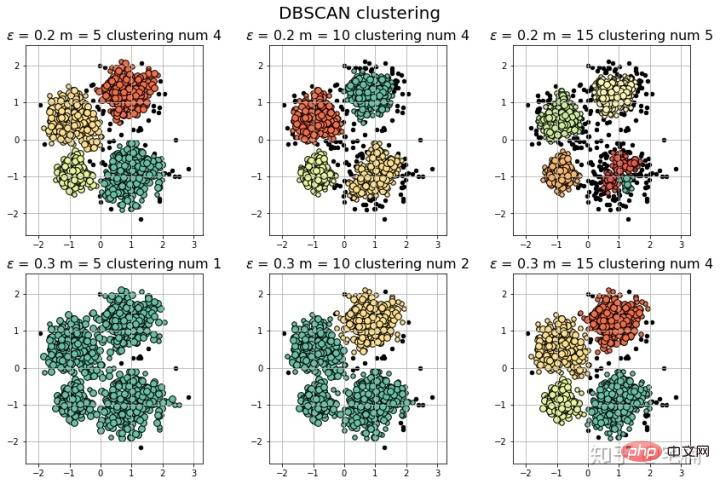 (Ich bin zu faul, das Markdown-Format zu konvertieren, also habe ich direkt einen Screenshot gemacht::>_<::)
#
# 参考https://blog.csdn.net/hb707934728/article/details/71515160
#
# 官方示例 https://scikit-learn.org/stable/auto_examples/cluster/plot_dbscan.html#sphx-glr-auto-examples-cluster-plot-dbscan-py

import numpy as np

import matplotlib.pyplot as plt
import matplotlib.colors

import sklearn.datasets as ds
from sklearn.cluster import DBSCAN
from sklearn.preprocessing import StandardScaler


def expand(a, b):
    d = (b - a) * 0.1
    return a-d, b+d


if __name__ == "__main__":
    N = 1000
    data = X_train_demo.values
    # 数据1的参数:(epsilon, min_sample)
    params = ((0.2, 5), (0.2, 10), (0.2, 15), (0.2, 20), (0.2, 25), (0.2, 30))

    plt.figure(figsize=(12, 8), facecolor='w')
    plt.suptitle(u'DBSCAN clustering', fontsize=20)

    for i in range(6):
        eps, min_samples = params[i]
        #参数含义:
        #eps:半径,表示以给定点P为中心的圆形邻域的范围
        #min_samples:以点P为中心的邻域内最少点的数量
        #如果满足,以点P为中心,半径为EPS的邻域内点的个数不少于MinPts,则称点P为核心点
        model = DBSCAN(eps=eps, min_samples=min_samples)
        model.fit(data)
        y_hat = model.labels_

        core_indices = np.zeros_like(y_hat, dtype=bool)  # 生成数据类型和数据shape和指定array一致的变量
        core_indices[model.core_sample_indices_] = True  # model.core_sample_indices_ border point位于y_hat中的下标

        # 统计总共有积累,其中为-1的为未分类样本
        y_unique = np.unique(y_hat)
        n_clusters = y_unique.size - (1 if -1 in y_hat else 0)
        print (y_unique, '聚类簇的个数为:', n_clusters)

        plt.subplot(2, 3, i+1) # 对第几个图绘制,2行3列,绘制第i+1个图
        # plt.cm.spectral https://blog.csdn.net/robin_Xu_shuai/article/details/79178857
        clrs = plt.cm.Spectral(np.linspace(0, 0.8, y_unique.size)) #用于给画图灰色
        for k, clr in zip(y_unique, clrs):
            cur = (y_hat == k)
            if k == -1:
                # 用于绘制未分类样本
                plt.scatter(data[cur, 0], data[cur, 1], s=20, c='k')
                continue
            # 绘制正常节点
            plt.scatter(data[cur, 0], data[cur, 1], s=30, c=clr, edgecolors='k')
            # 绘制边缘点
            plt.scatter(data[cur & core_indices][:, 0], data[cur & core_indices][:, 1], s=60, c=clr, marker='o', edgecolors='k')
        x1_min, x2_min = np.min(data, axis=0)
        x1_max, x2_max = np.max(data, axis=0)
        x1_min, x1_max = expand(x1_min, x1_max)
        x2_min, x2_max = expand(x2_min, x2_max)
        plt.xlim((x1_min, x1_max))
        plt.ylim((x2_min, x2_max))
        plt.grid(True)
        plt.title(u'$epsilon$ = %.1f m = %d clustering num %d'%(eps, min_samples, n_clusters), fontsize=14)
    plt.tight_layout()
    plt.subplots_adjust(top=0.9)
plt.show()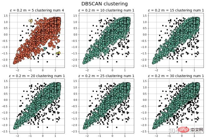 3
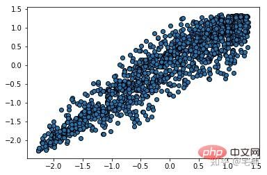
3 from sklearn.cluster import DBSCAN from sklearn import metrics data = X_train_demo.values eps, min_samples = 0.2, 10 # eps为领域的大小,min_samples为领域内最小点的个数 model = DBSCAN(eps=eps, min_samples=min_samples) # 构造分类器 model.fit(data) # 拟合 labels = model.labels_ # 获取类别标签,-1表示未分类 # 获取其中的core points core_indices = np.zeros_like(labels, dtype=bool) # 生成数据类型和数据shape和指定array一致的变量 core_indices[model.core_sample_indices_] = True # model.core_sample_indices_ border point位于labels中的下标 core_point = data[core_indices] # 获取非异常点 normal_point = data[labels>=0] # 绘制剔除了异常值后的图 plt.scatter(normal_point[:,0],normal_point[:,1],edgecolors='k') plt.show()
def filter_data(data0, params):
    from sklearn.cluster import DBSCAN
    from sklearn import metrics
    scaler = StandardScaler()
    scaler.fit(data0)
    data = scaler.transform(data0)

    eps, min_samples = params
    # eps为领域的大小,min_samples为领域内最小点的个数
    model = DBSCAN(eps=eps, min_samples=min_samples) # 构造分类器
    model.fit(data) # 拟合
    labels = model.labels_ # 获取类别标签,-1表示未分类
    # 获取其中的core points
    core_indices = np.zeros_like(labels, dtype=bool)  # 生成数据类型和数据shape和指定array一致的变量
    core_indices[model.core_sample_indices_] = True  # model.core_sample_indices_ border point位于labels中的下标
    core_point = data[core_indices]
    # 获取非异常点
    normal_point = data0[labels>=0]
return normal_pointVor dem Entfernen von Ausreißern
Die durchschnittliche Dichte der Probenpunkte um einen Probenpunkt herum ist höher als die Dichte des Probenpunkts. Je größer das Verhältnis größer als 1 ist, desto kleiner ist die Dichte am Ort des Punktes als die Dichte am Ort der umgebenden Proben.
# 轮廓系数
metrics.silhouette_score(data, labels, metric='euclidean')
[out]0.13250260550638607
# Calinski-Harabaz Index 系数
metrics.calinski_harabaz_score(data, labels,)
[out]16.414158842632794
# reference:https://scikit-learn.org/stable/auto_examples/svm/plot_oneclass.html#sphx-glr-auto-examples-svm-plot-oneclass-py

import numpy as np
import matplotlib.pyplot as plt
import matplotlib.font_manager
from sklearn import svm

xx, yy = np.meshgrid(np.linspace(-5, 5, 500), np.linspace(-5, 5, 500))
# Generate train data
X = 0.3 * np.random.randn(100, 2)
X_train = np.r_[X + 2, X - 2]
# Generate some regular novel observations
X = 0.3 * np.random.randn(20, 2)
X_test = np.r_[X + 2, X - 2]
# Generate some abnormal novel observations
X_outliers = np.random.uniform(low=-4, high=4, size=(20, 2))

# fit the model
clf = svm.OneClassSVM(nu=0.1, kernel="rbf", gamma=0.1)
clf.fit(X_train)
y_pred_train = clf.predict(X_train)
y_pred_test = clf.predict(X_test)
y_pred_outliers = clf.predict(X_outliers)
n_error_train = y_pred_train[y_pred_train == -1].size
n_error_test = y_pred_test[y_pred_test == -1].size
n_error_outliers = y_pred_outliers[y_pred_outliers == 1].size

# plot the line, the points, and the nearest vectors to the plane
Z = clf.decision_function(np.c_[xx.ravel(), yy.ravel()])
Z = Z.reshape(xx.shape)

plt.title("Novelty Detection")
plt.contourf(xx, yy, Z, levels=np.linspace(Z.min(), 0, 7), cmap=plt.cm.PuBu)
a = plt.contour(xx, yy, Z, levels=[0], linewidths=2, colors='darkred')
plt.contourf(xx, yy, Z, levels=[0, Z.max()], colors='palevioletred')

s = 40
b1 = plt.scatter(X_train[:, 0], X_train[:, 1], c='white', s=s, edgecolors='k')
b2 = plt.scatter(X_test[:, 0], X_test[:, 1], c='blueviolet', s=s,
                 edgecolors='k')
c = plt.scatter(X_outliers[:, 0], X_outliers[:, 1], c='gold', s=s,
                edgecolors='k')
plt.axis('tight')
plt.xlim((-5, 5))
plt.ylim((-5, 5))
plt.legend([a.collections[0], b1, b2, c],
           ["learned frontier", "training observations",
            "new regular observations", "new abnormal observations"],
           loc="upper left",
           prop=matplotlib.font_manager.FontProperties(size=11))
plt.xlabel(
    "error train: %d/200 ; errors novel regular: %d/40 ; "
    "errors novel abnormal: %d/40"
    % (n_error_train, n_error_test, n_error_outliers))
plt.show()Vor dem Entfernen von Ausreißern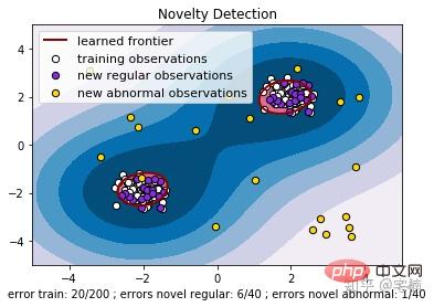
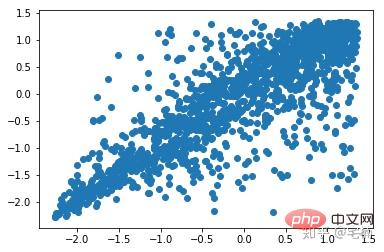
from sklearn import svm
X_train = X_train_demo.values
# 构造分类器
clf = svm.OneClassSVM(nu=0.2, kernel="rbf", gamma=0.2)
clf.fit(X_train)
# 预测,结果为-1或者1
labels = clf.predict(X_train)
# 分类分数
score = clf.decision_function(X_train) # 获取置信度
# 获取正常点
X_train_normal = X_train[labels>0]
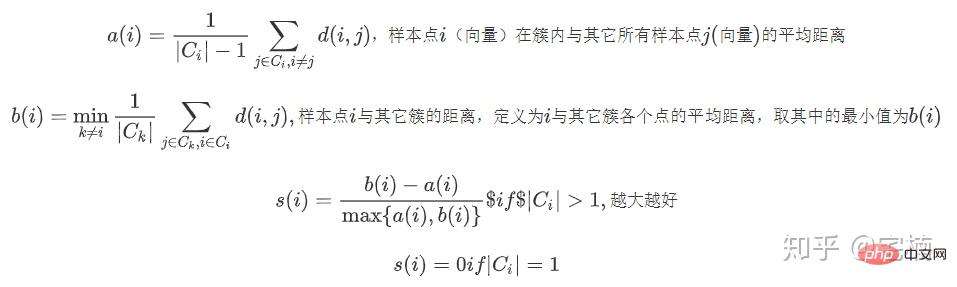
Das obige ist der detaillierte Inhalt vonWelche vier Methoden gibt es, um abnormale Daten zu beseitigen?. Für weitere Informationen folgen Sie bitte anderen verwandten Artikeln auf der PHP chinesischen Website!
 So laden Sie die heutigen Schlagzeilenvideos herunter und speichern sie
 Der Unterschied zwischen Windows-Ruhezustand und Ruhezustand
 So lösen Sie eine Java-Ausnahme beim Lesen großer Dateien
 Was ist Löwenzahn?
 Was sind die Vorteile des Java-Factory-Musters?
 Was bedeutet Linux?
 Einführung in SSL-Erkennungstools
 Welche Datensicherungssoftware gibt es?
 So entsperren Sie Android-Berechtigungsbeschränkungen


![[Web-Frontend] Node.js-Schnellstart](https://img.php.cn/upload/course/000/000/067/662b5d34ba7c0227.png)


