Detailliertes Tutorial zum Zeichnen dreidimensionaler Diagramme in Python

Dieser Artikel vermittelt Ihnen relevantes Wissen über Python Normalerweise verwenden wir Python zum Zeichnen zweidimensionaler Ebenendiagramme, aber manchmal müssen wir auch dreidimensionale Szenendiagramme zeichnen. Im Folgenden werden die relevanten Informationen zu Python zum Zeichnen dreidimensionaler Diagramme vorgestellt Diagramme. Ich hoffe, es hilft allen.

【Verwandte Empfehlung: Python3-Video-Tutorial】

Dieser Artikel fasst nur die grundlegendsten Zeichenmethoden zusammen.

1. Initialisierung

Es wird davon ausgegangen, dass das Matplotlib-Toolpaket installiert wurde.

Verwenden Sie matplotlib.figure.Figure, um einen Rahmen zu erstellen:

import matplotlib.pyplot as plt
from mpl_toolkits.mplot3d import Axes3D
fig = plt.figure()
ax = fig.add_subplot(111, projection='3d')

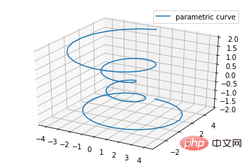
2. Liniendiagramme

Grundlegende Verwendung:

ax.plot(x,y,z,label=' ')

Code:

import matplotlib as mpl
from mpl_toolkits.mplot3d import Axes3D
import numpy as np
import matplotlib.pyplot as plt
 
mpl.rcParams['legend.fontsize'] = 10
 
fig = plt.figure()
ax = fig.gca(projection='3d')
theta = np.linspace(-4 * np.pi, 4 * np.pi, 100)
z = np.linspace(-2, 2, 100)
r = z**2 + 1
x = r * np.sin(theta)
y = r * np.cos(theta)
ax.plot(x, y, z, label='parametric curve')
ax.legend()
 
plt.show()

3. Streudiagramme s)

Grundlegende Verwendung:

ax.scatter(xs, ys, zs, s=20, c=None, depthshade=True, *args, *kwargs)

• xs,ys,zs: Eingabedaten;
• s: Größe des Streupunkts
• c: Farbe, z. B. c = 'r' ist rot;
• Depthshase: Transparenz, True ist transparent, der Standardwert ist True, False ist undurchsichtig.
• *Argumente usw. sind erweiterte Variablen, z. B. „maker = ‚o‘“, dann hat das Streuungsergebnis die Form von „o“

Code:

from mpl_toolkits.mplot3d import Axes3D
import matplotlib.pyplot as plt
import numpy as np
 
 
def randrange(n, vmin, vmax):
    '''
    Helper function to make an array of random numbers having shape (n, )
    with each number distributed Uniform(vmin, vmax).
    '''
    return (vmax - vmin)*np.random.rand(n) + vmin
 
fig = plt.figure()
ax = fig.add_subplot(111, projection='3d')
 
n = 100
 
# For each set of style and range settings, plot n random points in the box
# defined by x in [23, 32], y in [0, 100], z in [zlow, zhigh].
for c, m, zlow, zhigh in [('r', 'o', -50, -25), ('b', '^', -30, -5)]:
    xs = randrange(n, 23, 32)
    ys = randrange(n, 0, 100)
    zs = randrange(n, zlow, zhigh)
    ax.scatter(xs, ys, zs, c=c, marker=m)
 
ax.set_xlabel('X Label')
ax.set_ylabel('Y Label')
ax.set_zlabel('Z Label')
 
plt.show()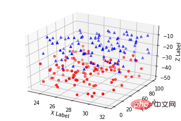

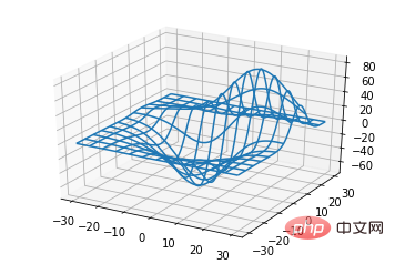
4. Zeilenblock Diagramm (Drahtmodelldiagramme)

Grundlegende Verwendung:

ax.plot_wireframe(X, Y, Z, *args, **kwargs)

• X, Y, Z: Eingabedaten
• rstride: Zeilenschrittlänge
• cstride: Spaltenschrittlänge
• rcount: Obergrenze der Zeilennummer
• ccount: Obergrenze Begrenzung der Spaltenanzahl

Code:

from mpl_toolkits.mplot3d import axes3d
import matplotlib.pyplot as plt
 
 
fig = plt.figure()
ax = fig.add_subplot(111, projection='3d')
 
# Grab some test data.
X, Y, Z = axes3d.get_test_data(0.05)
 
# Plot a basic wireframe.
ax.plot_wireframe(X, Y, Z, rstride=10, cstride=10)
 
plt.show()

5. Oberflächendiagramme

Grundlegende Verwendung:

ax.plot_surface(X, Y, Z, *args, **kwargs)

• Farbe: Oberflächenfarbe
• cmap: Ebene
Code:

from mpl_toolkits.mplot3d import Axes3D
import matplotlib.pyplot as plt
from matplotlib import cm
from matplotlib.ticker import LinearLocator, FormatStrFormatter
import numpy as np
 
 
fig = plt.figure()
ax = fig.gca(projection='3d')
 
# Make data.
X = np.arange(-5, 5, 0.25)
Y = np.arange(-5, 5, 0.25)
X, Y = np.meshgrid(X, Y)
R = np.sqrt(X**2 + Y**2)
Z = np.sin(R)
 
# Plot the surface.
surf = ax.plot_surface(X, Y, Z, cmap=cm.coolwarm,
                       linewidth=0, antialiased=False)
 
# Customize the z axis.
ax.set_zlim(-1.01, 1.01)
ax.zaxis.set_major_locator(LinearLocator(10))
ax.zaxis.set_major_formatter(FormatStrFormatter('%.02f'))
 
# Add a color bar which maps values to colors.
fig.colorbar(surf, shrink=0.5, aspect=5)
 
plt.show()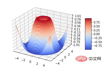

6. Dreiflächendiagramme

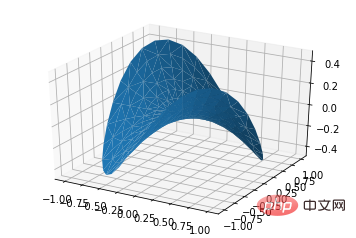
Grundlegende Verwendung:

ax.plot_trisurf(*args, **kwargs)

X, Y, Z: Daten.

• Andere Parameter sind ähnlich zum Oberflächenplot
Code:

from mpl_toolkits.mplot3d import Axes3D
import matplotlib.pyplot as plt
import numpy as np
 
 
n_radii = 8
n_angles = 36
 
# Make radii and angles spaces (radius r=0 omitted to eliminate duplication).
radii = np.linspace(0.125, 1.0, n_radii)
angles = np.linspace(0, 2*np.pi, n_angles, endpoint=False)
 
# Repeat all angles for each radius.
angles = np.repeat(angles[..., np.newaxis], n_radii, axis=1)
 
# Convert polar (radii, angles) coords to cartesian (x, y) coords.
# (0, 0) is manually added at this stage,  so there will be no duplicate
# points in the (x, y) plane.
x = np.append(0, (radii*np.cos(angles)).flatten())
y = np.append(0, (radii*np.sin(angles)).flatten())
 
# Compute z to make the pringle surface.
z = np.sin(-x*y)
 
fig = plt.figure()
ax = fig.gca(projection='3d')
 
ax.plot_trisurf(x, y, z, linewidth=0.2, antialiased=True)
 
plt.show()

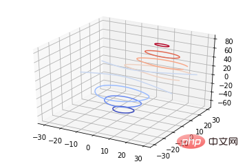
7. Konturdiagramme

Grundlegende Verwendung:

ax.contour(X, Y, Z, *args, **kwargs)

Code:

from mpl_toolkits.mplot3d import axes3d
import matplotlib.pyplot as plt
from matplotlib import cm
 
fig = plt.figure()
ax = fig.add_subplot(111, projection='3d')
X, Y, Z = axes3d.get_test_data(0.05)
cset = ax.contour(X, Y, Z, cmap=cm.coolwarm)
ax.clabel(cset, fontsize=9, inline=1)
 
plt.show()

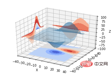
Zweidimensionale Konturen. Es kann auch dreidimensional gezeichnet werden Oberflächenkarte:

Code:

from mpl_toolkits.mplot3d import axes3d
from mpl_toolkits.mplot3d import axes3d
import matplotlib.pyplot as plt
from matplotlib import cm
 
fig = plt.figure()
ax = fig.gca(projection='3d')
X, Y, Z = axes3d.get_test_data(0.05)
ax.plot_surface(X, Y, Z, rstride=8, cstride=8, alpha=0.3)
cset = ax.contour(X, Y, Z, zdir='z', offset=-100, cmap=cm.coolwarm)
cset = ax.contour(X, Y, Z, zdir='x', offset=-40, cmap=cm.coolwarm)
cset = ax.contour(X, Y, Z, zdir='y', offset=40, cmap=cm.coolwarm)
 
ax.set_xlabel('X')
ax.set_xlim(-40, 40)
ax.set_ylabel('Y')
ax.set_ylim(-40, 40)
ax.set_zlabel('Z')
ax.set_zlim(-100, 100)
 
plt.show()

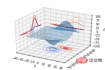Es kann auch die Projektion dreidimensionaler Konturen auf eine zweidimensionale Ebene sein:

Code:

from mpl_toolkits.mplot3d import axes3d
import matplotlib.pyplot as plt
from matplotlib import cm
 
fig = plt.figure()
ax = fig.gca(projection='3d')
X, Y, Z = axes3d.get_test_data(0.05)
ax.plot_surface(X, Y, Z, rstride=8, cstride=8, alpha=0.3)
cset = ax.contourf(X, Y, Z, zdir='z', offset=-100, cmap=cm.coolwarm)
cset = ax.contourf(X, Y, Z, zdir='x', offset=-40, cmap=cm.coolwarm)
cset = ax.contourf(X, Y, Z, zdir='y', offset=40, cmap=cm.coolwarm)
 
ax.set_xlabel('X')
ax.set_xlim(-40, 40)
ax.set_ylabel('Y')
ax.set_ylim(-40, 40)
ax.set_zlabel('Z')
ax.set_zlim(-100, 100)
 
plt.show()

ax.bar(left, height, zs=0, zdir='z', *args, **kwargs

8. Balkendiagramme (Bild)

Einfach Verwendung:

from mpl_toolkits.mplot3d import Axes3D
import matplotlib.pyplot as plt
import numpy as np
 
fig = plt.figure()
ax = fig.add_subplot(111, projection='3d')
for c, z in zip(['r', 'g', 'b', 'y'], [30, 20, 10, 0]):
    xs = np.arange(20)
    ys = np.random.rand(20)
 
    # You can provide either a single color or an array. To demonstrate this,
    # the first bar of each set will be colored cyan.
    cs = [c] * len(xs)
    cs[0] = 'c'
    ax.bar(xs, ys, zs=z, zdir='y', color=cs, alpha=0.8)
 
ax.set_xlabel('X')
ax.set_ylabel('Y')
ax.set_zlabel('Z')
 
plt.show()

• x, y, zs = z, Daten
• zdir: Die Richtung der Planarisierung des Balkendiagramms, die anhand des Codes im Detail verstanden werden kann.

Code:

from mpl_toolkits.mplot3d import Axes3D
import numpy as np
import matplotlib.pyplot as plt
 
fig = plt.figure()
ax = fig.gca(projection='3d')
 
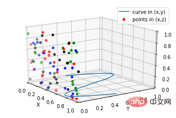
# Plot a sin curve using the x and y axes.
x = np.linspace(0, 1, 100)
y = np.sin(x * 2 * np.pi) / 2 + 0.5
ax.plot(x, y, zs=0, zdir='z', label='curve in (x,y)')
 
# Plot scatterplot data (20 2D points per colour) on the x and z axes.
colors = ('r', 'g', 'b', 'k')
x = np.random.sample(20*len(colors))
y = np.random.sample(20*len(colors))
c_list = []
for c in colors:
    c_list.append([c]*20)
# By using zdir='y', the y value of these points is fixed to the zs value 0
# and the (x,y) points are plotted on the x and z axes.
ax.scatter(x, y, zs=0, zdir='y', c=c_list, label='points in (x,z)')
 
# Make legend, set axes limits and labels
ax.legend()
ax.set_xlim(0, 1)
ax.set_ylim(0, 1)
ax.set_zlim(0, 1)
ax.set_xlabel('X')
ax.set_ylabel('Y')
ax.set_zlabel('Z')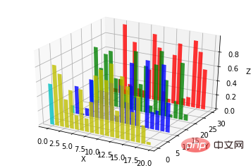

9. Subplot (Subplot)

A-unterschiedliche 2D-Grafiken, verteilt im 3D-Raum. Tatsächlich ist der Projektionsraum nicht leer, entsprechender Code:

subplot(2,2,1)
subplot(2,2,2)
subplot(2,2,[3,4])

B-Subplot-Verwendung

Der Unterschied zu MATLAB besteht darin, dass bei einem Vier-Subplot-Effekt, wie zum Beispiel:

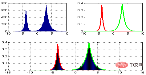
MATLAB:

subplot(2,2,1)
subplot(2,2,2)
subplot(2,1,2)

Python:

import matplotlib.pyplot as plt
from mpl_toolkits.mplot3d.axes3d import Axes3D, get_test_data
from matplotlib import cm
import numpy as np
 
 
# set up a figure twice as wide as it is tall
fig = plt.figure(figsize=plt.figaspect(0.5))
 
#===============
#  First subplot
#===============
# set up the axes for the first plot
ax = fig.add_subplot(2, 2, 1, projection='3d')
 
# plot a 3D surface like in the example mplot3d/surface3d_demo
X = np.arange(-5, 5, 0.25)
Y = np.arange(-5, 5, 0.25)
X, Y = np.meshgrid(X, Y)
R = np.sqrt(X**2 + Y**2)
Z = np.sin(R)
surf = ax.plot_surface(X, Y, Z, rstride=1, cstride=1, cmap=cm.coolwarm,
                       linewidth=0, antialiased=False)
ax.set_zlim(-1.01, 1.01)
fig.colorbar(surf, shrink=0.5, aspect=10)
 
#===============
# Second subplot
#===============
# set up the axes for the second plot
ax = fig.add_subplot(2,1,2, projection='3d')
 
# plot a 3D wireframe like in the example mplot3d/wire3d_demo
X, Y, Z = get_test_data(0.05)
ax.plot_wireframe(X, Y, Z, rstride=10, cstride=10)
 
plt.show()

Code:

from mpl_toolkits.mplot3d import Axes3D
import matplotlib.pyplot as plt
 
 
fig = plt.figure()
ax = fig.gca(projection='3d')
 
# Demo 1: zdir
zdirs = (None, 'x', 'y', 'z', (1, 1, 0), (1, 1, 1))
xs = (1, 4, 4, 9, 4, 1)
ys = (2, 5, 8, 10, 1, 2)
zs = (10, 3, 8, 9, 1, 8)
 
for zdir, x, y, z in zip(zdirs, xs, ys, zs):
    label = '(%d, %d, %d), dir=%s' % (x, y, z, zdir)
    ax.text(x, y, z, label, zdir)
 
# Demo 2: color
ax.text(9, 0, 0, "red", color='red')
 
# Demo 3: text2D
# Placement 0, 0 would be the bottom left, 1, 1 would be the top right.
ax.text2D(0.05, 0.95, "2D Text", transform=ax.transAxes)
 
# Tweaking display region and labels
ax.set_xlim(0, 10)
ax.set_ylim(0, 10)
ax.set_zlim(0, 10)
ax.set_xlabel('X axis')
ax.set_ylabel('Y axis')
ax.set_zlabel('Z axis')
 
plt.show()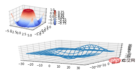

Ergänzung:

Grundlegende Verwendung von Textkommentaren:

Code:

rrreee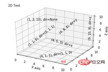

[Verwandte Empfehlungen: Python3-Video-Tutorial ]

Das obige ist der detaillierte Inhalt vonDetailliertes Tutorial zum Zeichnen dreidimensionaler Diagramme in Python. Für weitere Informationen folgen Sie bitte anderen verwandten Artikeln auf der PHP chinesischen Website!