So implementieren Sie einen Gradientenabstieg, um die logistische Regression in Python zu lösen

Lineare Regression

1. Die Definition der linearen Regressionsfunktion

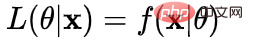
Wahrscheinlichkeitsfunktion: gegebener gemeinsamer Stichprobenwert Zufallsfunktion : Welche Art von Parametern sind in Kombination mit unseren Daten genau die wahren Werte

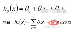
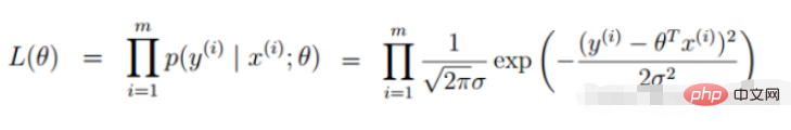
2. Lineare Regressionswahrscheinlichkeitsfunktion

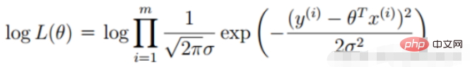
Log-Wahrscheinlichkeit:

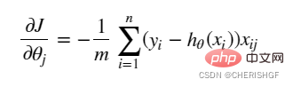
3. Lineare Regressionszielfunktion

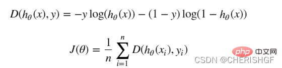
(Fehlerausdruck, unser Ziel ist es, den Fehler zwischen dem wahren Wert und dem vorhergesagten Wert zu minimieren )

(Die Ableitung ist 0, um den Extremwert zu erhalten, und die Parameter der Funktion werden erhalten)

Logistische Regression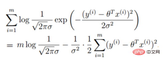

Logistische Regression Es dient dazu, dem Ergebnis der linearen Regression eine Ebene der Sigmoidfunktion hinzuzufügen

1. Logistische Regressionsfunktion

wird

eingeführt eine Gradientenabstiegsaufgabe, und die logistische Regressionszielfunktion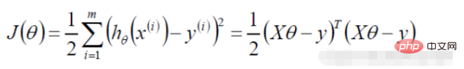

wird durch die Gradientenabstiegsmethode gelöst

Mein Verständnis besteht darin, die Parameter durch Ableitung zu aktualisieren, nach Erreichen einer bestimmten Bedingung anzuhalten und eine annähernd optimale Lösung zu erhalten

Code-Implementierung

Sigmoidfunktion

def sigmoid(z):    
   return 1 / (1 + np.exp(-z))

Vorhersagefunktion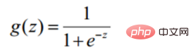

def model(X, theta):    
    return sigmoid(np.dot(X, theta.T))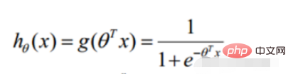

Zielfunktion

def cost(X, y, theta):    
     left = np.multiply(-y, np.log(model(X, theta)))    
     right = np.multiply(1 - y, np.log(1 - model(X, theta)))    
     return np.sum(left - right) / (len(X))

Gradient

def gradient(X, y, theta):    
  grad = np.zeros(theta.shape)    
  error = (model(X, theta)- y).ravel()    
  for j in range(len(theta.ravel())): #for each parmeter        
     term = np.multiply(error, X[:,j])        
     grad[0, j] = np.sum(term) / len(X)    
   return grad

Strategie zum Stoppen des Gradientenabstiegs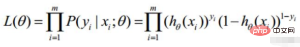

STOP_ITER = 0
STOP_COST = 1
STOP_GRAD = 2
 
def stopCriterion(type, value, threshold):
    # 设定三种不同的停止策略
    if type == STOP_ITER:  # 设定迭代次数
        return value > threshold
    elif type == STOP_COST:  # 根据损失值停止
        return abs(value[-1] - value[-2]) < threshold
    elif type == STOP_GRAD:  # 根据梯度变化停止
        return np.linalg.norm(value) < threshold

Beispielumbildung

import numpy.random
#洗牌
def shuffleData(data):
    np.random.shuffle(data)
    cols = data.shape[1]
    X = data[:, 0:cols-1]
    y = data[:, cols-1:]
    return X, y

Gradientenabstiegslösung

def descent(data, theta, batchSize, stopType, thresh, alpha):
    # 梯度下降求解
 
    init_time = time.time()
    i = 0  # 迭代次数
    k = 0  # batch
    X, y = shuffleData(data)
    grad = np.zeros(theta.shape)  # 计算的梯度
    costs = [cost(X, y, theta)]  # 损失值
 
    while True:
        grad = gradient(X[k:k + batchSize], y[k:k + batchSize], theta)
        k += batchSize  # 取batch数量个数据
        if k >= n:
            k = 0
            X, y = shuffleData(data)  # 重新洗牌
        theta = theta - alpha * grad  # 参数更新
        costs.append(cost(X, y, theta))  # 计算新的损失
        i += 1
 
        if stopType == STOP_ITER:
            value = i
        elif stopType == STOP_COST:
            value = costs
        elif stopType == STOP_GRAD:
            value = grad
        if stopCriterion(stopType, value, thresh): break
 
    return theta, i - 1, costs, grad, time.time() - init_time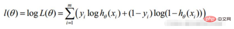

Vollständiger Code

import numpy as np
import pandas as pd
import matplotlib.pyplot as plt
import os
import numpy.random
import time
 
 
def sigmoid(z):
    return 1 / (1 + np.exp(-z))
 
 
def model(X, theta):
    return sigmoid(np.dot(X, theta.T))
 
 
def cost(X, y, theta):
    left = np.multiply(-y, np.log(model(X, theta)))
    right = np.multiply(1 - y, np.log(1 - model(X, theta)))
    return np.sum(left - right) / (len(X))
 
 
def gradient(X, y, theta):
    grad = np.zeros(theta.shape)
    error = (model(X, theta) - y).ravel()
    for j in range(len(theta.ravel())):  # for each parmeter
        term = np.multiply(error, X[:, j])
        grad[0, j] = np.sum(term) / len(X)
    return grad
 
 
STOP_ITER = 0
STOP_COST = 1
STOP_GRAD = 2
 
 
def stopCriterion(type, value, threshold):
    # 设定三种不同的停止策略
    if type == STOP_ITER:  # 设定迭代次数
        return value > threshold
    elif type == STOP_COST:  # 根据损失值停止
        return abs(value[-1] - value[-2]) < threshold
    elif type == STOP_GRAD:  # 根据梯度变化停止
        return np.linalg.norm(value) < threshold
 
 
# 洗牌
def shuffleData(data):
    np.random.shuffle(data)
    cols = data.shape[1]
    X = data[:, 0:cols - 1]
    y = data[:, cols - 1:]
    return X, y
 
 
def descent(data, theta, batchSize, stopType, thresh, alpha):
    # 梯度下降求解
 
    init_time = time.time()
    i = 0  # 迭代次数
    k = 0  # batch
    X, y = shuffleData(data)
    grad = np.zeros(theta.shape)  # 计算的梯度
    costs = [cost(X, y, theta)]  # 损失值
 
    while True:
        grad = gradient(X[k:k + batchSize], y[k:k + batchSize], theta)
        k += batchSize  # 取batch数量个数据
        if k >= n:
            k = 0
            X, y = shuffleData(data)  # 重新洗牌
        theta = theta - alpha * grad  # 参数更新
        costs.append(cost(X, y, theta))  # 计算新的损失
        i += 1
 
        if stopType == STOP_ITER:
            value = i
        elif stopType == STOP_COST:
            value = costs
        elif stopType == STOP_GRAD:
            value = grad
        if stopCriterion(stopType, value, thresh): break
 
    return theta, i - 1, costs, grad, time.time() - init_time
 
 
def runExpe(data, theta, batchSize, stopType, thresh, alpha):
    # import pdb
    # pdb.set_trace()
    theta, iter, costs, grad, dur = descent(data, theta, batchSize, stopType, thresh, alpha)
    name = "Original" if (data[:, 1] > 2).sum() > 1 else "Scaled"
    name += " data - learning rate: {} - ".format(alpha)
    if batchSize == n:
        strDescType = "Gradient"  # 批量梯度下降
    elif batchSize == 1:
        strDescType = "Stochastic"  # 随机梯度下降
    else:
        strDescType = "Mini-batch ({})".format(batchSize)  # 小批量梯度下降
    name += strDescType + " descent - Stop: "
    if stopType == STOP_ITER:
        strStop = "{} iterations".format(thresh)
    elif stopType == STOP_COST:
        strStop = "costs change < {}".format(thresh)
    else:
        strStop = "gradient norm < {}".format(thresh)
    name += strStop
    print("***{}\nTheta: {} - Iter: {} - Last cost: {:03.2f} - Duration: {:03.2f}s".format(
        name, theta, iter, costs[-1], dur))
    fig, ax = plt.subplots(figsize=(12, 4))
    ax.plot(np.arange(len(costs)), costs, 'r')
    ax.set_xlabel('Iterations')
    ax.set_ylabel('Cost')
    ax.set_title(name.upper() + ' - Error vs. Iteration')
    return theta
 
 
path = 'data' + os.sep + 'LogiReg_data.txt'
pdData = pd.read_csv(path, header=None, names=['Exam 1', 'Exam 2', 'Admitted'])
positive = pdData[pdData['Admitted'] == 1]
negative = pdData[pdData['Admitted'] == 0]
 
# 画图观察样本情况
fig, ax = plt.subplots(figsize=(10, 5))
ax.scatter(positive['Exam 1'], positive['Exam 2'], s=30, c='b', marker='o', label='Admitted')
ax.scatter(negative['Exam 1'], negative['Exam 2'], s=30, c='r', marker='x', label='Not Admitted')
ax.legend()
ax.set_xlabel('Exam 1 Score')
ax.set_ylabel('Exam 2 Score')
 
pdData.insert(0, 'Ones', 1)
 
# 划分训练数据与标签
orig_data = pdData.values
cols = orig_data.shape[1]
X = orig_data[:, 0:cols - 1]
y = orig_data[:, cols - 1:cols]
# 设置初始参数0
theta = np.zeros([1, 3])
 
# 选择的梯度下降方法是基于所有样本的
n = 100
runExpe(orig_data, theta, n, STOP_ITER, thresh=5000, alpha=0.000001)
runExpe(orig_data, theta, n, STOP_COST, thresh=0.000001, alpha=0.001)
runExpe(orig_data, theta, n, STOP_GRAD, thresh=0.05, alpha=0.001)
runExpe(orig_data, theta, 1, STOP_ITER, thresh=5000, alpha=0.001)
runExpe(orig_data, theta, 1, STOP_ITER, thresh=15000, alpha=0.000002)
runExpe(orig_data, theta, 16, STOP_ITER, thresh=15000, alpha=0.001)
 
from sklearn import preprocessing as pp
 
# 数据预处理
scaled_data = orig_data.copy()
scaled_data[:, 1:3] = pp.scale(orig_data[:, 1:3])
 
runExpe(scaled_data, theta, n, STOP_ITER, thresh=5000, alpha=0.001)
runExpe(scaled_data, theta, n, STOP_GRAD, thresh=0.02, alpha=0.001)
theta = runExpe(scaled_data, theta, 1, STOP_GRAD, thresh=0.002 / 5, alpha=0.001)
runExpe(scaled_data, theta, 16, STOP_GRAD, thresh=0.002 * 2, alpha=0.001)
 
 
# 设定阈值
def predict(X, theta):
    return [1 if x >= 0.5 else 0 for x in model(X, theta)]
 
 
# 计算精度
scaled_X = scaled_data[:, :3]
y = scaled_data[:, 3]
predictions = predict(scaled_X, theta)
correct = [1 if ((a == 1 and b == 1) or (a == 0 and b == 0)) else 0 for (a, b) in zip(predictions, y)]
accuracy = (sum(map(int, correct)) % len(correct))
print('accuracy = {0}%'.format(accuracy))

Vorteile und Nachteile der logistischen Regression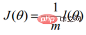

Vorteile

Die Form ist einfach und die Interpretierbarkeit des Modells ist sehr gut. Anhand der Gewichtung des Merkmals können wir die Auswirkung verschiedener Merkmale auf das Endergebnis erkennen. Wenn der Gewichtungswert eines bestimmten Merkmals relativ hoch ist, hat dieses Merkmal einen größeren Einfluss auf das Endergebnis.

Das Modell funktioniert gut. Dies ist im Engineering akzeptabel (als Basis), wenn das Feature-Engineering gut durchgeführt wird, wird der Effekt nicht allzu schlimm sein, und das Feature-Engineering kann parallel entwickelt werden, was die Entwicklung erheblich beschleunigt.

Trainingsgeschwindigkeit ist schneller. Bei der Klassifizierung hängt der Rechenaufwand nur von der Anzahl der Features ab. Darüber hinaus ist der SGD der verteilten Optimierung der logistischen Regression relativ ausgereift, und die Trainingsgeschwindigkeit kann durch Heap-Maschinen weiter verbessert werden, sodass wir in kurzer Zeit mehrere Versionen des Modells iterieren können.

Es beansprucht nur wenig Ressourcen, insbesondere Speicher. Denn nur die Merkmalswerte jeder Dimension müssen gespeichert werden.

Bequem zum Anpassen der Ausgabeergebnisse. Die logistische Regression kann leicht das endgültige Klassifizierungsergebnis erhalten, da die Ausgabe die Wahrscheinlichkeitsbewertung jeder Stichprobe ist und wir diese Wahrscheinlichkeitsbewertungen leicht abschneiden können, dh den Schwellenwert aufteilen (diejenigen, die über einem bestimmten Schwellenwert liegen, werden in eine Kategorie klassifiziert). diejenigen, die kleiner als ein bestimmter Schwellenwert sind, sind eine Kategorie).

Nachteile

Die Genauigkeit ist nicht sehr hoch. Da die Form sehr einfach ist (sehr ähnlich einem linearen Modell), ist es schwierig, die wahre Verteilung der Daten anzupassen.

Es ist schwierig, mit dem Problem des Datenungleichgewichts umzugehen. Beispiel: Wenn wir uns mit einem Problem befassen, bei dem positive und negative Stichproben sehr unausgeglichen sind, beispielsweise wenn das Verhältnis von positiven und negativen Stichproben 10.000:1 beträgt, können wir auch den Wert der Verlustfunktion festlegen kleiner. Als Klassifikator ist seine Fähigkeit, positive und negative Proben zu unterscheiden, jedoch nicht sehr gut.

Die Verarbeitung nichtlinearer Daten ist problematischer. Die logistische Regression kann ohne Einführung anderer Methoden nur linear trennbare Daten oder darüber hinaus binäre Klassifizierungsprobleme verarbeiten.

Die logistische Regression selbst kann keine Features filtern. Manchmal verwenden wir gbdt zum Filtern von Features und verwenden dann die logistische Regression.

Das obige ist der detaillierte Inhalt vonSo implementieren Sie einen Gradientenabstieg, um die logistische Regression in Python zu lösen. Für weitere Informationen folgen Sie bitte anderen verwandten Artikeln auf der PHP chinesischen Website!