 Technology peripherals
 AI
AI
 Overview of path planning: based on sampling, search, and optimization, all done!
Overview of path planning: based on sampling, search, and optimization, all done!
1 Overview of decision control and motion planning
Currently decision control methods can be divided into three categories: sequential planning, behavior-aware planning, and end-to-end planning .
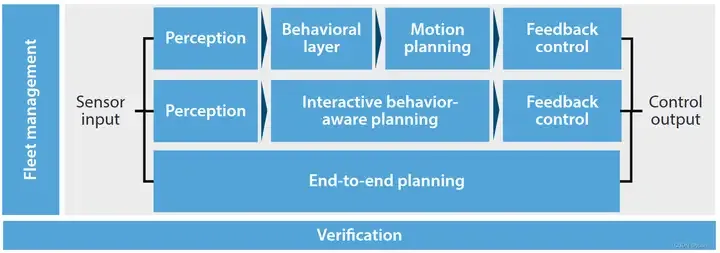
- sequential planning: the most traditional method, perception, decision-making and control The levels of each part are relatively clear;
- behavior-aware planning: Compared with the first type, the highlight is the introduction of human-machine co-driving, vehicle-road collaboration, and vehicle risk estimation of the external dynamic environment;
- End-to-end planning: DL and DRL technology uses a large amount of data training to obtain the relationship from sensory information such as images to vehicle control inputs such as steering wheel angle. It is one of the most popular methods nowadays.
This article will introduce sequential planning, follow the entire decision-making control sequence and describe the perception control process of autonomous vehicles. Finally, it will briefly summarize the issues to be solved mentioned above. question.
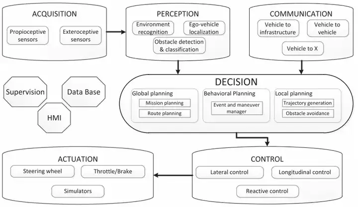
Control architecture for automated vehicles
2 Overview of path planning
The process of sequential planning is briefly summarized asPath Planning->Decision-making process->Vehicle Control, the path planning described in this article belongs to the first and third steps.
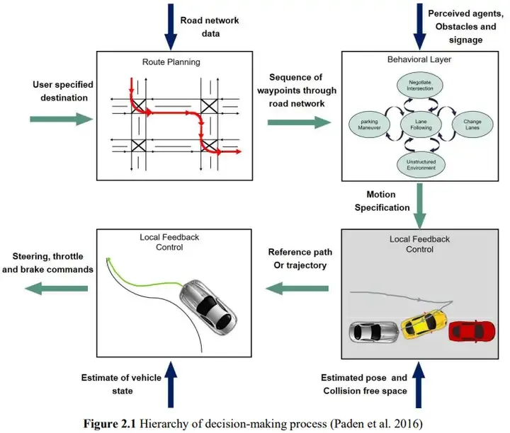
https://www.php.cn/link/aa7d66ed4b1c618962d406535c4d282a
On the issue of motion trajectory generation of unmanned vehicles , there are direct trajectory generation method and path-speed decomposition method. Compared with the first method, path-speed is less difficult, so it is more commonly used.
2.1 Types of path planning
Path planning can be divided into four major categories: sampling-based algorithms represented by PRM and RRT, Algorithms based on search represented by A* and D*, trajectory generation algorithms based on interpolationfitting represented by β-splines, and MPC represented by Optimal control algorithm for local path planning. This section will explain them one by one in the order mentioned above:
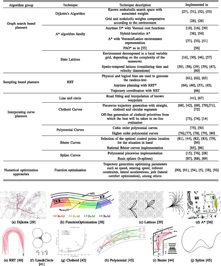
A Review of Motion Planning Techniques for Automated Vehicles
2.2 Advantages and Disadvantages of Path Planning Algorithms
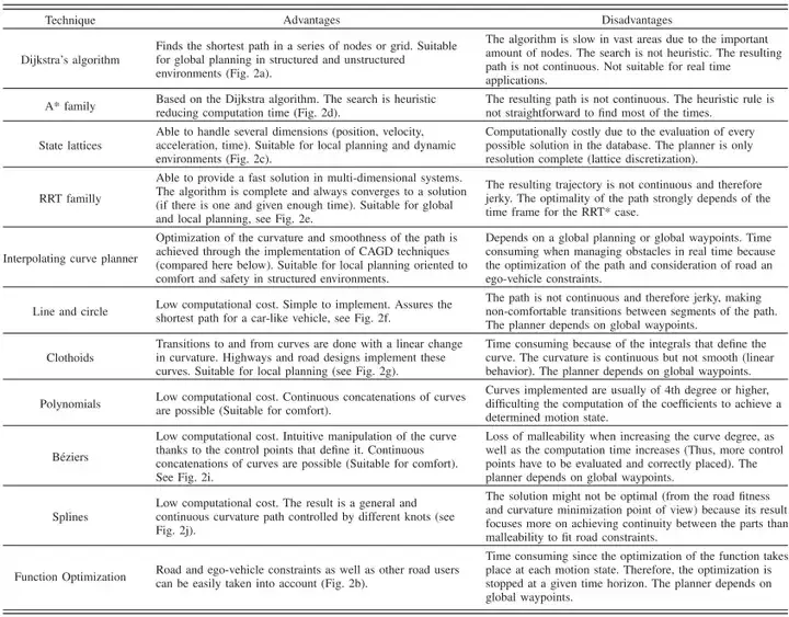
3 Path planning method
3.1 Sampling-based algorithm
3.1.1 Basic algorithm PRM and RRT
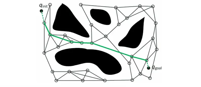
(1) PRM
PRM algorithm (Probabilistic Road Map) . PRM mainly consists of two steps, one is the learning stage, and the other is the query stage.
The first step, the learning stage: uniformly and randomly sample n points in the safe area in the state space, and delete the points where the samples fall on the obstacles, and then connect the adjacent points and perform collision detection. , eliminate the connections that are not collision-free, and finally obtain a connected graph.
The second step, the query stage: for a given pair of initial and target states, use the sampling nodes and continuity constructed in the previous step, and use the graph search method (Dijkstra or A*) to find a feasible path.
After completing the PRM construction, it can be used to solve motion planning problems in different initial and target states, but this feature is unnecessary for unmanned vehicle motion planning. In addition, PRM requires precise connections between states, which is very difficult for motion planning problems with complex differential constraints.
(2) RRT
RRT (Rapidly-exploring Random Tree) algorithm. RRT actually represents a series of algorithms based on the idea of randomly growing trees. It is currently the most widely used algorithm with the most optimized variants in the field of robotics.
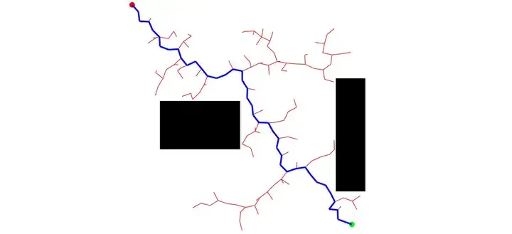
① Tree initialization: Initialize the node set and edge set of the tree. The node set only contains the initial state and the edge set is empty;
② Tree growth: Randomly sample the state space. When the sampling point falls in the safe area of the state space, select the node closest to the sampling point in the current tree and extend it to the sampling point; if the generated trajectory does not If it collides with an obstacle, the trajectory is added to the edge set of the tree, and the end point of the trajectory is added to the node set of the tree
③ Repeat step ② until it is expanded to the target state set. Compared with PRM, there is no In terms of graphs, RRT constructs a tree structure with the initial state as the root node and the target state as the leaf node. For different initial and target states, different trees need to be constructed.
RRT does not require precise connections between states and is more suitable for solving motion dynamics problems such as unmanned vehicle motion planning.
3.1.2 Problems and Solutions of Sampling Method
Solution efficiency and whether it is the optimal solution. The reason why PRM and RRT have probabilistic completeness is that they will traverse almost all positions in the configuration space.
(1) Solving efficiency
In terms of improving solving efficiency, the core idea of optimizing RRT is to guide the tree to the open area, that is, try to stay away from obstacles and avoid repeated checks of nodes at obstacles to improve efficiency. Main solution:
① Uniform sampling
The standard RRT algorithm samples the state spaceuniformly and randomly, and the nodes in the current tree obtain The probability of expansion is proportional to the area of its Voronoi region, so the tree will grow towards the empty area of the state space, evenly filling the free area of the state space.
The RRT-connect algorithm simultaneously constructs two trees starting from the initial state and the target state. When the two trees grow together then a feasible solution is found. Go-biaing inserts the target state at a certain proportion in the random sampling sequence, guiding the tree to expand toward the target state, speeding up the solution speed, and improving the solution quality.
Heuristic RRT uses a heuristic function to increase the probability of sampling nodes with low expansion costs and calculate the cost of each node in the tree. However, in complex environments, the definition of the cost function is difficult. In order to solve this problem For one problem, the f-biased sampling method first discretizes the state space into a grid, and then uses the Dijkstra algorithm to calculate the cost on each grid. The cost value of the points in the area of the grid is equal to this value, thereby constructing a heuristic formula function.
② Optimize distance measurement
Distance is used to measure the cost of the path between two configurations, assists in generating a heuristic cost function, and guides the direction of the tree. However, distance calculation is difficult when obstacles are considered. The definition of distance in motion planning adopts a definition similar to Euclidean distance. RG-RRT (rechability guided RRT) can eliminate the impact of inaccurate distance on RRT exploration ability. It needs to calculate the reachable set of nodes in the tree. When the distance from the sampling point to the node is greater than the reachable set of the node, distance, the node may be selected for expansion.
③ Reduce the number of collision checks
One of the efficiency bottlenecks of the collision check sampling method, the usual approach is to discretize the path at equal distances, Then perform a collision check on the configuration at each point. resolution complete RRT obtains the probability of expansion by reducing nodes close to obstacles. It discretizes the input space and only uses it once for a certain node input; if the trajectory corresponding to a certain input collides with an obstacle , then a penalty value is added to the node. The higher the penalty value, the smaller the probability of the node being expanded. Dynamic domain RRT and adaptive dynamic domain RRT limit the sampling area to the local space where the current tree is located to prevent nodes close to obstacles from repeated expansion failures and improve algorithm efficiency.
④ Improve real-time performance
Anytime RRT first quickly builds an RRT, obtains a feasible solution and records its cost, and then continues sampling, but it will only help reduce the feasibility The node with the solution cost is inserted into the tree, thereby gradually obtaining a better feasible solution. Replanning decomposes the entire planning task into a number of equal-time sub-task sequences, and plans the next task while executing the current task.
(2) There are mainly the following methods to solve the optimality problem:
RGG algorithm (random geometric graph): According to the random geometric graph theory, the standard PRM and RRT is an improved PRM, RRG and RRT algorithm with asymptotic optimal properties. It randomly samples n points in the state space and connects the points whose distance is less than r(n) to form RGG. . RRT* Algorithm: Introduce the "reconnection" step based on RRG to check whether the newly inserted node as the parent node of its adjacent point will reduce the cost of its adjacent points. If it does, remove the adjacent points. Click the original parent-child relationship and use the current insertion point as its parent node. This is the RRT* algorithm.
LBT-RRT algorithm: A large number of node connections and local adjustments make PRM and RRT very inefficient. The LBT-RRT algorithm combines the RRG and RRT* algorithms to obtain higher efficiency on the premise of obtaining asymptotic optimality.
3.2 Search-based algorithm
The basic idea is to discretize the state spacein a certain way into a graph, and then use each A heuristic search algorithmsearchesfeasible solutionsor evenoptimal solutions, this category algorithm is relatively mature.
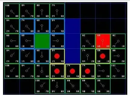
The basis of the search-based algorithm is the state lattice. The state lattice is the discretization of the state space, consisting of the state node and the movement starting from the node to the adjacent node. Composed of primitives, one state node can be transformed to another state node through its motion primitives. The state lattice converts the original continuous state space into a search graph. The motion planning problem becomes searching for a series of motion primitives that transform the initial state to the target state in the graph. After constructing the state lattice, you can use graph search algorithm to search for the optimal trajectory.
3.2.1 Construction of basic algorithms Dijkstra and A*
Dijkstra algorithm traverses the entire configuration space, finds the distance between each two grids, and finally selects The shortest path from the starting point to the target point has a very low efficiency due to its breadth-first nature. On the basis of this algorithm, adding a heuristic function, that is, the distance from the searched node to the target node, and searching again based on this can avoid The inefficiency caused by global search is the A* algorithm, as shown in the figure below, the red is the search area.
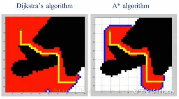
Figure 6: Comparison of the effects of A* and Dijkstra algorithms
3.2.2 Problems and suggestions of search methods
Same as sampling-based algorithms, this type of algorithm also needs to be optimized for efficiency and optimality.
In terms of improving efficiency, A* itself is a static planning algorithm. An extension of the A* algorithm is weighted A*, which further guides the search direction to the target node by increasing the weight of the heuristic function, improving the search speed. It is fast, but it is easy to fall into local minima and cannot guarantee the global optimal solution.
For moving vehicles, using A*’s derivative algorithm D (dynamic A) can greatly improve efficiency. Also based on dynamic programming is LPA. This algorithm can handle the situation where the cost of the motion primitives of the state grid is time-varying. When the environment changes, a new optimal plan can be planned by re-searching a smaller number of nodes. path. Developed on the basis of LPA , D*-Lite can achieve the same results as D*, but with higher efficiency.
When searching for optimal solutions, ARA* is an Anytime search algorithm developed on the basis of Weighted A*. It calls the Weighted A* algorithm multiple times and narrows down the heuristics with each call. The weight of the formula function allows the algorithm to quickly find a feasible solution. By introducing the set INCONS, each cycle can continue to use the information of the previous cycle to optimize the path and gradually approach the optimal solution.
On the issue of balancing algorithm efficiency and optimality, Sandin aine et al. proposed the MHA* algorithm, which introduced multiple heuristic functions to ensure that one of the heuristic functions can find the optimal solution when used alone. , so that by coordinating the path costs generated by different heuristic functions, the efficiency and optimality of the algorithm can be taken into account. DMHA generates appropriate heuristic functions online and in real time based on MHA, thereby avoiding the local minimum problem.
3.3 Algorithm based on interpolation fitting
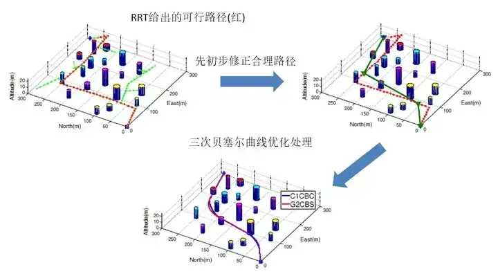
The algorithm based on interpolation fitting can be defined as: according to a known The series is used to describe the point set of the road map. By using data interpolation and curve fitting, the path that the smart car will travel can be created. Provide better continuity and higher derivability. The specific method is as follows:
Dubins curve and Reeds and Sheep (RS) curve are the shortest paths connecting any two points in the configuration space, corresponding to the situations without reversing and with reversing respectively. They are all composed of arcs of maximum curvature and straight lines. There is a curvature discontinuity at the connection between the arc and the straight line. When an actual vehicle travels on such a curve, it must stop and adjust the steering wheel at the discontinuity of curvature to continue driving.
Polynomial interpolation curve is the most commonly used method. It can set polynomial coefficients by meeting the requirements of nodes and obtain better continuous differentiability. Fourth-order polynomials It is often used in longitudinal constraint control, fifth-order polynomials are often used in lateral constraint control, and third-order polynomials are also used in overtaking trajectories.
Spline curve has a closed expression and can easily ensure curvature continuity. β-spline curves can achieve curvature continuity, and cubic Bezier curves can ensure the continuity and boundedness of curvature, and the amount of calculation is relatively small. The η^3 curve [43] is a seven-degree spline curve, which has very good properties: continuity of curvature and continuity of curvature derivatives, which is very meaningful for high-speed vehicles.
3.4 Algorithms based on optimal control
Algorithms based on optimal control are classified into path planning, mainly because the MPC can perform local path planning For obstacle avoidance, in addition, the main function of MPC is trajectory tracking. In addition to the necessary dynamics and kinematic constraints, the issues it considers should also consider comfort, uncertainty of sensory information, and workshop in the future. communication uncertainty, and the driver can also be included in the control loop during local trajectory planning. The above-mentioned uncertainty issues and incorporating the driver into the control loop will be discussed in Section 4. Regarding the study of MPC, we mainly start from two aspects: optimization theory and engineering practice. For the former, I recommend Convex Optimization Algorithms by Dimitri P. Bertsekas and Model Predictive Control: Theory, Computation, and Design by James B. Rawlings. In the Chinese field, teacher Liu Haoyang’s optimization book personally feels that it is relatively clear and easy to understand. For the latter, first of all, Teacher Gong Jianwei’s self-driving MPC book is strongly recommended. There were problems with the demo in the old version of the book, but they were all solved in the new version.
There are many types of prediction models used by MPC: such as convolutional neural network, fuzzy control, state space, etc. Among them, the most commonly used is the state space method. MPC can be briefly expressed as: when the necessary dynamics, kinematics, etc. constraints are met, the optimal solution of the model is solved through numerical means. The optimal solution is the control variable of the state equation, such as the steering wheel angle, etc., and Apply the control quantity to the car model to obtain the required state quantities, such as speed, acceleration, coordinates, etc.
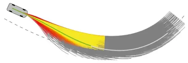
It can be seen from the above description that the key to MPC lies in the establishment and solution of the model. How to equivalently simplify the establishment of the model and improve the efficiency of the solution is the top priority. The vehicle will take different trajectories under different control inputs, and each trajectory corresponds to an objective function value. The unmanned vehicle will use a solving algorithm to find the control quantity corresponding to the minimum objective function value, and apply it to the vehicle. As shown in the figure below:
In order to reduce the difficulty of modeling, artificial potential energy field models are also used for modeling. The basic idea of artificial potential energy fields is similar to electric fields. On the road Obstacles are analogous to charges in an electric field that are of a different polarity than the source of the field. The potential energy at obstacles (dynamic, static) is higher, and the unmanned vehicle will move toward a low potential energy position.
4 Open source project
Recommend an open source project CppRobotics:
- Path Planning
- Dijkstra
- A Star
- RRT
- Dynamic Window Approach
- Model Predictive Trajectory Generator
- Cubic Spline Planner
- State Lattice Planner
- Frenet Frame Trajectory
5 Learning method
The learning context for entry into new fields is: Engineering, Theory and Vision Troika go hand in hand, taking path planning as an example:
5.1 Engineering
refers to understanding each path planning algorithm Content, while understanding the content of each algorithm from breadth, while learning the details of each algorithm from depth. Regarding algorithms in the field of path planning, there is currently no comprehensive tutorial, but Gong Jianwei's NMPC motion planning can be a reference.
5.2 Theory
refers to understanding the mathematical principles that support the operation of these algorithms and the reasons why these algorithms are generated (mathematical perspective).
- Constructing the objective function and constraint conditions while seeking the extreme value to obtain the optimal control quantity (path), which belongs to Optimization theory;
- is solving the optimal problem The common numerical solution methods such as Newton's method and steepest descent method when controlling quantities essentially come from numerically solving algebraic equations and belong to numerical analysis;
- What you see during the solution process The obtained derivative Jacobian matrix, vector norms in judgment conditions, etc. are essentially the solution of one-dimensional numerical calculations to high dimensions, which belongs to matrix theory.
5.3 Vision
refers to understanding the main applications of path planning in scientific research and enterprises, using scientific research documents and results reports, etc.
6 Summary
This article introduces the outline of current path planning and understands the current path planning methods. The content is very complicated, and it is difficult to learn it all in a short period of time without practical application orientation. You can only focus on learning when needed.
The above is the detailed content of Overview of path planning: based on sampling, search, and optimization, all done!. For more information, please follow other related articles on the PHP Chinese website!

Hot AI Tools

Undresser.AI Undress
AI-powered app for creating realistic nude photos

AI Clothes Remover
Online AI tool for removing clothes from photos.

Undress AI Tool
Undress images for free

Clothoff.io
AI clothes remover

Video Face Swap
Swap faces in any video effortlessly with our completely free AI face swap tool!

Hot Article

Hot Tools

Notepad++7.3.1
Easy-to-use and free code editor

SublimeText3 Chinese version
Chinese version, very easy to use

Zend Studio 13.0.1
Powerful PHP integrated development environment

Dreamweaver CS6
Visual web development tools

SublimeText3 Mac version
God-level code editing software (SublimeText3)

Hot Topics
 1388
1388
 52
52
 Why is Gaussian Splatting so popular in autonomous driving that NeRF is starting to be abandoned?
Jan 17, 2024 pm 02:57 PM
Written above & the author’s personal understanding Three-dimensional Gaussiansplatting (3DGS) is a transformative technology that has emerged in the fields of explicit radiation fields and computer graphics in recent years. This innovative method is characterized by the use of millions of 3D Gaussians, which is very different from the neural radiation field (NeRF) method, which mainly uses an implicit coordinate-based model to map spatial coordinates to pixel values. With its explicit scene representation and differentiable rendering algorithms, 3DGS not only guarantees real-time rendering capabilities, but also introduces an unprecedented level of control and scene editing. This positions 3DGS as a potential game-changer for next-generation 3D reconstruction and representation. To this end, we provide a systematic overview of the latest developments and concerns in the field of 3DGS for the first time.
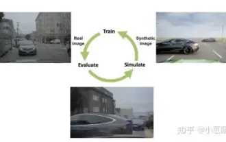 How to solve the long tail problem in autonomous driving scenarios?
Jun 02, 2024 pm 02:44 PM
Yesterday during the interview, I was asked whether I had done any long-tail related questions, so I thought I would give a brief summary. The long-tail problem of autonomous driving refers to edge cases in autonomous vehicles, that is, possible scenarios with a low probability of occurrence. The perceived long-tail problem is one of the main reasons currently limiting the operational design domain of single-vehicle intelligent autonomous vehicles. The underlying architecture and most technical issues of autonomous driving have been solved, and the remaining 5% of long-tail problems have gradually become the key to restricting the development of autonomous driving. These problems include a variety of fragmented scenarios, extreme situations, and unpredictable human behavior. The "long tail" of edge scenarios in autonomous driving refers to edge cases in autonomous vehicles (AVs). Edge cases are possible scenarios with a low probability of occurrence. these rare events
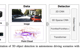 Choose camera or lidar? A recent review on achieving robust 3D object detection
Jan 26, 2024 am 11:18 AM
0.Written in front&& Personal understanding that autonomous driving systems rely on advanced perception, decision-making and control technologies, by using various sensors (such as cameras, lidar, radar, etc.) to perceive the surrounding environment, and using algorithms and models for real-time analysis and decision-making. This enables vehicles to recognize road signs, detect and track other vehicles, predict pedestrian behavior, etc., thereby safely operating and adapting to complex traffic environments. This technology is currently attracting widespread attention and is considered an important development area in the future of transportation. one. But what makes autonomous driving difficult is figuring out how to make the car understand what's going on around it. This requires that the three-dimensional object detection algorithm in the autonomous driving system can accurately perceive and describe objects in the surrounding environment, including their locations,
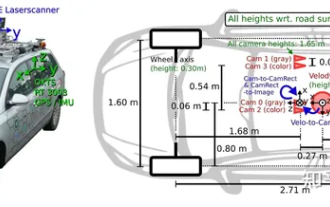 Have you really mastered coordinate system conversion? Multi-sensor issues that are inseparable from autonomous driving
Oct 12, 2023 am 11:21 AM
The first pilot and key article mainly introduces several commonly used coordinate systems in autonomous driving technology, and how to complete the correlation and conversion between them, and finally build a unified environment model. The focus here is to understand the conversion from vehicle to camera rigid body (external parameters), camera to image conversion (internal parameters), and image to pixel unit conversion. The conversion from 3D to 2D will have corresponding distortion, translation, etc. Key points: The vehicle coordinate system and the camera body coordinate system need to be rewritten: the plane coordinate system and the pixel coordinate system. Difficulty: image distortion must be considered. Both de-distortion and distortion addition are compensated on the image plane. 2. Introduction There are four vision systems in total. Coordinate system: pixel plane coordinate system (u, v), image coordinate system (x, y), camera coordinate system () and world coordinate system (). There is a relationship between each coordinate system,
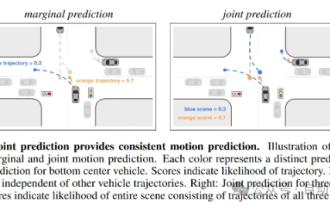 This article is enough for you to read about autonomous driving and trajectory prediction!
Feb 28, 2024 pm 07:20 PM
Trajectory prediction plays an important role in autonomous driving. Autonomous driving trajectory prediction refers to predicting the future driving trajectory of the vehicle by analyzing various data during the vehicle's driving process. As the core module of autonomous driving, the quality of trajectory prediction is crucial to downstream planning control. The trajectory prediction task has a rich technology stack and requires familiarity with autonomous driving dynamic/static perception, high-precision maps, lane lines, neural network architecture (CNN&GNN&Transformer) skills, etc. It is very difficult to get started! Many fans hope to get started with trajectory prediction as soon as possible and avoid pitfalls. Today I will take stock of some common problems and introductory learning methods for trajectory prediction! Introductory related knowledge 1. Are the preview papers in order? A: Look at the survey first, p
 Let's talk about end-to-end and next-generation autonomous driving systems, as well as some misunderstandings about end-to-end autonomous driving?
Apr 15, 2024 pm 04:13 PM
In the past month, due to some well-known reasons, I have had very intensive exchanges with various teachers and classmates in the industry. An inevitable topic in the exchange is naturally end-to-end and the popular Tesla FSDV12. I would like to take this opportunity to sort out some of my thoughts and opinions at this moment for your reference and discussion. How to define an end-to-end autonomous driving system, and what problems should be expected to be solved end-to-end? According to the most traditional definition, an end-to-end system refers to a system that inputs raw information from sensors and directly outputs variables of concern to the task. For example, in image recognition, CNN can be called end-to-end compared to the traditional feature extractor + classifier method. In autonomous driving tasks, input data from various sensors (camera/LiDAR
 SIMPL: A simple and efficient multi-agent motion prediction benchmark for autonomous driving
Feb 20, 2024 am 11:48 AM
Original title: SIMPL: ASimpleandEfficientMulti-agentMotionPredictionBaselineforAutonomousDriving Paper link: https://arxiv.org/pdf/2402.02519.pdf Code link: https://github.com/HKUST-Aerial-Robotics/SIMPL Author unit: Hong Kong University of Science and Technology DJI Paper idea: This paper proposes a simple and efficient motion prediction baseline (SIMPL) for autonomous vehicles. Compared with traditional agent-cent
 FisheyeDetNet: the first target detection algorithm based on fisheye camera
Apr 26, 2024 am 11:37 AM
Target detection is a relatively mature problem in autonomous driving systems, among which pedestrian detection is one of the earliest algorithms to be deployed. Very comprehensive research has been carried out in most papers. However, distance perception using fisheye cameras for surround view is relatively less studied. Due to large radial distortion, standard bounding box representation is difficult to implement in fisheye cameras. To alleviate the above description, we explore extended bounding box, ellipse, and general polygon designs into polar/angular representations and define an instance segmentation mIOU metric to analyze these representations. The proposed model fisheyeDetNet with polygonal shape outperforms other models and simultaneously achieves 49.5% mAP on the Valeo fisheye camera dataset for autonomous driving


