 Technology peripherals
 AI
AI
 CVPR\'24 Oral | A look at the past and present life of the pure sparse point cloud detector SAFDNet!
CVPR\'24 Oral | A look at the past and present life of the pure sparse point cloud detector SAFDNet!
Written before&The author’s personal understanding
3D point cloud object detection is crucial to autonomous driving perception, how to efficiently learn features from sparse point cloud data Representation is a key challenge in the field of 3D point cloud object detection. In this article, we will introduce the HEDNet published by the team in NeurIPS 2023 and SAFDNet in CVPR 2024. HEDNet focuses on solving the problem that existing sparse convolutional neural networks are difficult to capture the dependencies between long-distance features, while SAFDNet is built based on HEDNet. Pure sparse point cloud detector. In point cloud object detection, traditional methods often rely on hand-designed feature extractors, which have limited effectiveness when processing sparse point cloud data. In recent years, deep learning-based methods have made significant progress in this field. HEDNet uses convolutional neural networks to extract features from sparse point cloud data, and solves key problems in sparse point cloud data through a specific network structure, such as capturing the dependencies between long-distance features. This method is in the paper of NeurIPS 2023
Previous life-HEDNet
Research background
Mainstream methods usually treat unstructured The point cloud is converted into regular elements and features are extracted using a sparse convolutional neural network or Transformer. Most existing sparse convolutional neural networks are mainly built by stacking submanifold manifold residual (SSR) modules. Each SSR module contains two submanifold convolutions using small convolution kernels. (Submanifold Sparse, SS) convolution. However, submanifold convolution requires the sparsity of input and output feature maps to remain constant, which hinders the model from capturing the dependencies between distant features. One possible solution is to replace the submanifold convolution in the SSR module with a regular sparse (RS) convolution. However, as the network depth increases, this results in lower feature map sparsity, resulting in a substantial increase in computational cost. Some research attempts to use sparse convolutional neural networks or Transformers based on large convolution kernels to capture the dependencies between long-distance features, but these methods either do not bring improvement in accuracy or require higher computational costs. In summary, we still lack a method that can efficiently capture the dependencies between distant features.
Method introduction
SSR module and RSR module
In order to improve the efficiency of the model, the existing 3D point cloud object detection Most of them use sparse convolution to extract features. Sparse convolution mainly includes RS convolution and SS convolution. RS convolution will spread sparse features to adjacent areas during the calculation process, thus reducing the sparsity of the feature map. In contrast, SS convolution keeps the sparsity of the input and output feature maps unchanged. Due to the computational cost of RS convolution by reducing the sparsity of feature maps, RS convolution is usually only used for feature map downsampling in existing methods. On the other hand, most element-based methods build sparse convolutional neural networks by stacking SSR modules to extract point cloud features. Each SSR module contains two SS convolutions and a skip connection that fuses input and output features.
Figure 1(a) shows the structure of a single SSR module. The valid feature in the figure refers to the non-zero feature, while the value of the empty feature is zero, which means that the position does not originally contain a point cloud. We define the sparsity of a feature map as the ratio of the area occupied by empty features to the total area of the feature map. In the SSR module, the input feature map is converted by two SS convolutions to obtain the output feature map. At the same time, the information of the input feature map is directly integrated into the output feature map through skip connection (Skip conn.). SS convolution only processes valid features to ensure that the output feature map of the SSR module has the same sparsity as the input feature map. However, such a design hinders information interaction between disconnected features. For example, the feature points marked by asterisks in the top feature map cannot receive information from the three feature points marked by red triangles outside the red dotted box in the bottom feature map, which limits the model's ability to model dependencies between long-distance features. Ability.
 Figure 1 Structural comparison of SSR, RSR and SED modules
In response to the above problems, a possible solution is to replace the SS convolution in the SSR module with RS convolution. Capture dependencies between distant features. We call this modified module the Regular Sparse Residual (RSR) module, and its structure is shown in Figure 1(b). In the figure, the expanded feature is an empty feature in the neighborhood of valid features. RS convolution processes both effective features and features to be diffused, and its convolution kernel center traverses these feature areas. This design results in a lower sparsity in the output feature image. Stacked RS convolution will reduce the sparsity of the feature map more quickly, resulting in a significant reduction in model efficiency. This is also the reason why existing methods usually use RS convolution for feature downsampling. Here, it is more appropriate for us to translate expanded features into features to be diffused.
SED module and DED module
The design goal of the SED module is to overcome the limitations of the SSR module. The SED module shortens the spatial distance between distant features through feature downsampling, and at the same time restores the lost detailed information through multi-scale feature fusion. Figure 1(c) shows an example of an SED module with two feature scales. This module first uses a 3x3 RS convolution with a stride of 3 for feature downsampling (Down). After feature downsampling, the disconnected effective features in the bottom feature map are integrated into the middle feature map and adjacent effective features. Then, the interaction between effective features is achieved by using an SSR module to extract features on the intermediate feature map. Finally, the intermediate feature maps are upsampled (UP) to match the resolution of the input feature maps. It is worth noting that here only the sample features are upsampled to the regions corresponding to valid features in the input feature map. Therefore, the SED module can maintain the sparsity of feature maps. The design goal of the SED module is to overcome the limitations of the SSR module. The SED module shortens the spatial distance between distant features through feature downsampling, and at the same time restores the lost detailed information through multi-scale feature fusion. Figure 1(c) shows an example of an SED module with two feature scales. This module first uses a 3x3 RS convolution with a stride of 3 for feature downsampling (Down). After feature downsampling, the disconnected effective features in the bottom feature map are integrated into the middle feature map and adjacent effective features. Then, the interaction between effective features is achieved by using an SSR module to extract features on the intermediate feature map. Finally, the intermediate feature maps are upsampled (UP) to match the resolution of the input feature maps. It is worth noting that here only the sample features are upsampled to the regions corresponding to valid features in the input feature map. Therefore, the SED module can maintain the sparsity of feature maps. The design goal of the SED module is to overcome the limitations of the SSR module
The SED module demonstrates a specific implementation of the SED module with three characteristic scales. The number in parentheses represents the ratio of the resolution of the corresponding feature map to the resolution of the input feature map. The SED module adopts an asymmetric codec structure, which uses the encoder to extract multi-scale features and gradually fuses the extracted multi-scale features through the decoder. The SED module uses RS convolution as the feature downsampling layer and sparse deconvolution as the feature upsampling layer. By using an encoder-decoder structure, the SED module facilitates information interaction between disconnected features in space, thereby enabling the model to capture dependencies between distant features.
 Figure 2 SED and DED module structures
On the other hand, the current mainstream 3D point cloud detectors mainly rely on object center features for prediction, but in sparse convolutional network extraction In the feature map, there may be holes in the center area of the object, especially on large objects. To solve this problem, we propose the DED module, whose structure is shown in Figure 2(b). The DED module has the same structure as the SED module, it replaces the SSR module in the SED module with a Dense Residual (DR) module, and replaces the RS convolution used for feature downsampling with DR with a stride of 2 module and replaces sparse deconvolution for feature upsampling with dense deconvolution. These designs enable the DED module to effectively diffuse sparse features toward the center area of the object.
HEDNet
Based on the SED module and the DED module, we propose the hierarchical codec network HEDNet. As shown in Figure 3, HEDNet extracts high-level sparse features through a 3D sparse backbone network, then diffuses the sparse features to the center area of the object through a 2D dense backbone network, and finally sends the features output by the 2D dense backbone network to the detection head for task prediction. . For the convenience of presentation, the feature map and subsequent feature downsampling layer are omitted in the figure. Macroscopically, HEDNet adopts a hierarchical network structure similar to SECOND, and the resolution of its feature maps gradually decreases; microscopically, HEDNet's core components SED module and DED module both adopt a codec structure. This is where the name HEDNet comes from.
 Figure 3 HEDNet overall framework
小Easter Egg
Why do we think of using the codec structure? In fact, HEDNet was inspired by our previous work CEDNet: A Cascade Encoder-Decoder Network for Dense Prediction (called CFNet before the name was changed). If you are interested, you can read our paper.
Experimental results
We compared the comprehensive performance of HEDNet with previously leading methods, and the results are shown in Figure 4. Compared with LargeKernel3D based on large convolution kernel CNN and DSVT-Voxel based on Transformer, HEDNet achieves better results in both detection accuracy and model inference speed. It is worth mentioning that compared with the previous state-of-the-art method DSVT, HEDNet achieves higher detection accuracy and increases model inference speed by 50%. More detailed results can be found in our paper.
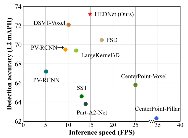
Figure 4 Comprehensive performance comparison on the Waymo Open data set
This life-SAFDNet
Research background
Voxel-based methods usually convert sparse voxel features into dense feature maps, and then extract features through dense convolutional neural networks for prediction. We call this type of detector hybrid detector, and its structure is shown in Figure 5(a). This type of method performs well in small-range (<75 meters) detection scenarios, but as the sensing range expands, the computational cost of using dense feature maps increases dramatically, limiting their use in large-range (>200 meters) detection scenarios. Applications. A possible solution is to build a pure sparse detector by removing the dense feature maps in existing hybrid detectors, but this will lead to a significant degradation in the detection performance of the model, as most hybrid detectors currently Prediction relies on object center features. When using pure sparse detectors to extract features, the center area of large objects is usually empty. This is the problem of missing object center features. Therefore, learning appropriate object representations is crucial for building purely sparse detectors.
Figure 5 Structural comparison of hybrid detector, FSDv1 and SAFDNet In order to solve the problem of missing object center features, FSDv1 (Figure 5(b)) first The original point cloud is divided into foreground points and background points, and then the foreground points are clustered through the center point voting mechanism, and instance features are extracted from each cluster for initial prediction, and finally further refined through the Group Correction Head. In order to reduce the inductive bias introduced by manual extraction of instance features, FSDv2 uses a virtual voxelization module to replace the instance clustering operation in FSDv1. The FSD series of methods are quite different from widely used detection frameworks such as CenterPoint, and introduce a large number of hyperparameters, making it challenging to deploy these methods in real scenarios. Different from the FSD series of methods, VoxelNeXt directly predicts based on the voxel features closest to the center of the object, but sacrifices detection accuracy.
So what does the pure sparse point cloud detector we want look like? First, the structure should be simple, so that it can be directly deployed into practical applications. An intuitive idea is to make minimal changes to build a pure sparse detector based on the currently widely used hybrid detector architecture such as CenterPoint; secondly, in terms of performance It must at least match the current leading hybrid detectors and be applicable to different ranges of detection scenarios.
Method IntroductionStarting from the above two requirements, we constructed a pure sparse 3D point cloud object detector SAFDNet based on HEDNet. Its macro structure is shown in Figure 5(c) ) shown. SAFDNet first uses a sparse voxel feature extractor to extract sparse point cloud features, and then uses an Adaptive Feature Diffusion (AFD) strategy and a 2D sparse convolutional neural network to diffuse the sparse features to the center area of the object to solve the problem of the center of the object. Missing features problem, and finally prediction based on sparse voxel features. SAFDNet can perform efficient calculations using only sparse features, and most of its structural design and hyperparameters are consistent with the baseline hybrid detectors, making it easy to adapt to actual application scenarios to replace existing hybrid detectors. The specific structure of SAFDNet is introduced below.
SAFDNet overall frameworkFigure 6 shows the overall framework of SAFDNet. Similar to existing hybrid detectors, SAFDNet mainly consists of three parts: a 3D sparse backbone network, a 2D sparse backbone network and a sparse detection head. The 3D sparse backbone network is used to extract 3D sparse voxel features and convert these features into 2D sparse BEV features. The 3D sparse backbone network uses the 3D-EDB module to promote information interaction between long-distance features (the 3D-EDB module is the SED module built based on 3D sparse convolution, and the 2D-EDB module below is similar). The 2D sparse backbone network receives the sparse BEV features output by the 3D sparse backbone network as input. It first classifies each voxel to determine whether the geometric center of each voxel falls within the object bounding box of a specific category or whether it belongs to the background area. Then, the sparse features are diffused to the center area of the object through the AFD operation and the 2D-EDB module. This part is the core component of SAFDNet. The sparse detection head makes predictions based on the sparse BEV features output by the 2D sparse backbone network. SAFDNet adopts the detection head design proposed by CenterPoint, and we made some adjustments to it to adapt to sparse features. Please see the paper for more details.
Figure 6 SAFDNet overall frameworkAdaptive Feature Diffusion (AFD)
Since the point cloud generated by lidar is mainly distributed on the surface of the object, using a pure sparse detector to extract features for prediction will face the lack of object center features question. So can the detector extract features closer to or located at the center of the object while maintaining feature sparsity as much as possible? An intuitive idea is to spread sparse features into neighboring voxels. Figure 6(a) shows an example of a sparse feature map. The red dot in the figure represents the center of the object. Each square represents a voxel. The dark orange squares are non-empty voxels whose geometric centers fall within the object bounding box. The dark blue squares are non-empty voxels whose geometric center falls outside the object's bounding box, and the white squares are empty voxels. Each non-empty voxel corresponds to a non-empty feature. Figure 7(b) is obtained by uniformly diffusing the non-empty features in Figure 7(a) to the neighborhood of KxK (K is 5). Diffused non-empty voxels are shown in light orange or light blue.
 Figure 7 Schematic diagram of uniform feature diffusion and adaptive feature diffusion
By analyzing the sparse feature map output by the 3D sparse backbone network, we observe that: (a) less than 10% The voxels fall within the bounding box of the object; (b) small objects usually have non-null features near or on their center voxel. This observation suggests that spreading all non-null features into the same size domain may be unnecessary, especially for voxels within small object bounding boxes and in background regions. Therefore, we propose an adaptive feature diffusion strategy that dynamically adjusts the diffusion range based on the location of voxel features. As shown in Figure 7(c), this strategy brings voxel features within the bounding box of large objects closer to the object center by allocating a larger diffusion range to these features, while at the same time by assigning voxel features within the bounding box of small objects and in the background area Voxel features are assigned a smaller diffusion range to maintain feature sparsity as much as possible. In order to implement this strategy, voxel classification (Voxel classification) is required to determine whether the geometric center of any non-empty voxel is within the bounding box of a specific category of objects or belongs to the background area. Please refer to the paper for more details on voxel classification. By using an adaptive feature diffusion strategy, the detector is able to maintain feature sparsity as much as possible, thereby benefiting from efficient computation of sparse features.
Main experimental results
We compared SAFDNet with the previous best methods in terms of comprehensive performance, and the results are shown in Figure 8. On the Waymo Open dataset with a smaller detection range, SAFDNet achieved comparable detection accuracy with the previous best pure sparse detector FSDv2 and our proposed hybrid detector HEDNet, but the inference speed of SAFDNet is 2 times that of FSDv2 and HEDNet 1.2 times. On the Argoverse2 data set with a large detection range, compared with the pure sparse detector FSDv2, SAFDNet improved the indicator mAP by 2.1%, and the inference speed reached 1.3 times that of FSDv2; compared with the hybrid detector HEDNet, SAFDNet improved The indicator mAP increased by 2.6%, and the inference speed reached 2.1 times that of HEDNet. In addition, when the detection range is large, the memory consumption of the hybrid detector HEDNet is much greater than that of the pure sparse detector. To sum up, SAFDNet is suitable for different ranges of detection scenarios and has excellent performance.
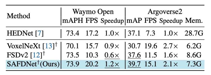
Figure 8 Main experimental results
Future work
SAFDNet is a pure sparse point cloud detector solution, so is there a problem with it? In fact, SAFDNet is just an intermediate product of our idea of a pure sparse detector. I think it is too violent and not concise and elegant enough. Please look forward to our follow-up work!
The codes of HEDNet and SAFDNet are open source and everyone is welcome to use them. Here is the link: https://github.com/zhanggang001/HEDNet
The above is the detailed content of CVPR\'24 Oral | A look at the past and present life of the pure sparse point cloud detector SAFDNet!. For more information, please follow other related articles on the PHP Chinese website!

Hot AI Tools

Undresser.AI Undress
AI-powered app for creating realistic nude photos

AI Clothes Remover
Online AI tool for removing clothes from photos.

Undress AI Tool
Undress images for free

Clothoff.io
AI clothes remover

Video Face Swap
Swap faces in any video effortlessly with our completely free AI face swap tool!

Hot Article

Hot Tools

Notepad++7.3.1
Easy-to-use and free code editor

SublimeText3 Chinese version
Chinese version, very easy to use

Zend Studio 13.0.1
Powerful PHP integrated development environment

Dreamweaver CS6
Visual web development tools

SublimeText3 Mac version
God-level code editing software (SublimeText3)

Hot Topics
 1664
1664
 14
14
 1423
1423
 52
52
 1317
1317
 25
25
 1268
1268
 29
29
 1243
1243
 24
24
 Why is Gaussian Splatting so popular in autonomous driving that NeRF is starting to be abandoned?
Jan 17, 2024 pm 02:57 PM
Written above & the author’s personal understanding Three-dimensional Gaussiansplatting (3DGS) is a transformative technology that has emerged in the fields of explicit radiation fields and computer graphics in recent years. This innovative method is characterized by the use of millions of 3D Gaussians, which is very different from the neural radiation field (NeRF) method, which mainly uses an implicit coordinate-based model to map spatial coordinates to pixel values. With its explicit scene representation and differentiable rendering algorithms, 3DGS not only guarantees real-time rendering capabilities, but also introduces an unprecedented level of control and scene editing. This positions 3DGS as a potential game-changer for next-generation 3D reconstruction and representation. To this end, we provide a systematic overview of the latest developments and concerns in the field of 3DGS for the first time.
 Python: How to create and visualize point clouds
May 02, 2023 pm 01:49 PM
1. Introduction Point cloud applications are everywhere: robots, self-driving cars, assistance systems, healthcare, etc. Point cloud is a 3D representation suitable for processing real-world data, especially when the geometry of the scene/object is required, such as the distance, shape and size of the object. A point cloud is a set of points that represent a real-world scene or an object in space. It is a discrete representation of geometric objects and scenes. In other words, point cloud PCD is a collection of n points, where each point Pi is represented by its 3D coordinates: Note that some other features can also be added to describe the point cloud, such as RGB color, normal, etc. For example, RGB colors can be added to provide color information. 2. Point cloud generation Point clouds usually use 3D scanners (laser scanners, time-of-flight scanners and structured light scanners)
 Learn about 3D Fluent emojis in Microsoft Teams
Apr 24, 2023 pm 10:28 PM
You must remember, especially if you are a Teams user, that Microsoft added a new batch of 3DFluent emojis to its work-focused video conferencing app. After Microsoft announced 3D emojis for Teams and Windows last year, the process has actually seen more than 1,800 existing emojis updated for the platform. This big idea and the launch of the 3DFluent emoji update for Teams was first promoted via an official blog post. Latest Teams update brings FluentEmojis to the app Microsoft says the updated 1,800 emojis will be available to us every day
 Updated Point Transformer: more efficient, faster and more powerful!
Jan 17, 2024 am 08:27 AM
Original title: PointTransformerV3: Simpler, Faster, Stronger Paper link: https://arxiv.org/pdf/2312.10035.pdf Code link: https://github.com/Pointcept/PointTransformerV3 Author unit: HKUSHAILabMPIPKUMIT Paper idea: This article is not intended to be published in Seeking innovation within the attention mechanism. Instead, it focuses on leveraging the power of scale to overcome existing trade-offs between accuracy and efficiency in the context of point cloud processing. Draw inspiration from recent advances in 3D large-scale representation learning,
 Using Python to implement point cloud ground detection
May 09, 2023 pm 05:28 PM
1. Computer Vision Coordinate Systems Before starting, it is important to understand the traditional coordinate systems in computer vision. This is followed by Open3D and Microsoft Kinect sensors. In computer vision, images are represented by a separate 2D coordinate system, where the x-axis points from left to right and the y-axis points up and down. For a camera, the origin of the 3D coordinate system is at the focus of the camera, with the x-axis pointing to the right, the y-axis pointing down, and the z-axis pointing forward. Computer Vision Coordinate System We first import the required Python library: importnumpyasnpimportopen3daso3d For better understanding, let us import the point cloud from the PLY file, using Open3D to create the default 3
 Choose camera or lidar? A recent review on achieving robust 3D object detection
Jan 26, 2024 am 11:18 AM
0.Written in front&& Personal understanding that autonomous driving systems rely on advanced perception, decision-making and control technologies, by using various sensors (such as cameras, lidar, radar, etc.) to perceive the surrounding environment, and using algorithms and models for real-time analysis and decision-making. This enables vehicles to recognize road signs, detect and track other vehicles, predict pedestrian behavior, etc., thereby safely operating and adapting to complex traffic environments. This technology is currently attracting widespread attention and is considered an important development area in the future of transportation. one. But what makes autonomous driving difficult is figuring out how to make the car understand what's going on around it. This requires that the three-dimensional object detection algorithm in the autonomous driving system can accurately perceive and describe objects in the surrounding environment, including their locations,
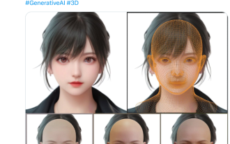 Get a virtual 3D wife in 30 seconds with a single card! Text to 3D generates a high-precision digital human with clear pore details, seamlessly connecting with Maya, Unity and other production tools
May 23, 2023 pm 02:34 PM
ChatGPT has injected a dose of chicken blood into the AI industry, and everything that was once unthinkable has become basic practice today. Text-to-3D, which continues to advance, is regarded as the next hotspot in the AIGC field after Diffusion (images) and GPT (text), and has received unprecedented attention. No, a product called ChatAvatar has been put into low-key public beta, quickly garnering over 700,000 views and attention, and was featured on Spacesoftheweek. △ChatAvatar will also support Imageto3D technology that generates 3D stylized characters from AI-generated single-perspective/multi-perspective original paintings. The 3D model generated by the current beta version has received widespread attention.
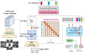 CLIP-BEVFormer: Explicitly supervise the BEVFormer structure to improve long-tail detection performance
Mar 26, 2024 pm 12:41 PM
Written above & the author’s personal understanding: At present, in the entire autonomous driving system, the perception module plays a vital role. The autonomous vehicle driving on the road can only obtain accurate perception results through the perception module. The downstream regulation and control module in the autonomous driving system makes timely and correct judgments and behavioral decisions. Currently, cars with autonomous driving functions are usually equipped with a variety of data information sensors including surround-view camera sensors, lidar sensors, and millimeter-wave radar sensors to collect information in different modalities to achieve accurate perception tasks. The BEV perception algorithm based on pure vision is favored by the industry because of its low hardware cost and easy deployment, and its output results can be easily applied to various downstream tasks.


