

Super strong! The top ten machine learning algorithms you must know


1. Linear regression
Linear regression is the simplest and most widely used method for predictive modeling One of the machine learning algorithms.
It is a supervised learning algorithm used to predict the value of a dependent variable based on one or more independent variables.
Definition
The core of linear regression is to fit a linear model based on observed data.
The linear model is represented by the following equation:
where
- is the dependent variable (The variable we want to predict)
- is the independent variable (the variable we use to predict)
- is the slope of the straight line
- is the y-axis intercept (the intersection of the straight line and the y-axis)
The linear regression algorithm involves finding the best path through the data points Fitting line. This is usually done by minimizing the squared difference between the observed and predicted values.
Evaluation Metrics
- Mean Square Error (MSE): The average of the squares of the measurement errors. The lower the value, the better.
- R-squared: Indicates the percentage of variation in the dependent variable that can be predicted from the independent variables. The closer to 1 the better.
from sklearn.datasets import load_diabetesfrom sklearn.model_selection import train_test_splitfrom sklearn.linear_model import LinearRegressionfrom sklearn.metrics import mean_squared_error, r2_score# Load the Diabetes datasetdiabetes = load_diabetes()X, y = diabetes.data, diabetes.target# Splitting the dataset into training and testing setsX_train, X_test, y_train, y_test = train_test_split(X, y, test_size=0.2, random_state=42)# Creating and training the Linear Regression modelmodel = LinearRegression()model.fit(X_train, y_train)# Predicting the test set resultsy_pred = model.predict(X_test)# Evaluating the modelmse = mean_squared_error(y_test, y_pred)r2 = r2_score(y_test, y_pred)print("MSE is:", mse)print("R2 score is:", r2)2. Logistic regression
Logistic regression is used for classification problems. It predicts the probability that a given data point belongs to a certain category, such as yes/no or 0/1.
Evaluation indicators
- Accuracy: Accuracy is the number of correctly predicted observations and the total number of observations The ratio.
- Precision and Recall: Precision is the ratio of correctly predicted positive observations to all expected positive observations. Recall is the ratio of correctly predicted positive observations to all actual observations.
- F1 Score: The balance between recall and precision.
from sklearn.datasets import load_breast_cancerfrom sklearn.linear_model import LogisticRegressionfrom sklearn.model_selection import train_test_splitfrom sklearn.metrics import accuracy_score, precision_score, recall_score, f1_score# Load the Breast Cancer datasetbreast_cancer = load_breast_cancer()X, y = breast_cancer.data, breast_cancer.target# Splitting the dataset into training and testing setsX_train, X_test, y_train, y_test = train_test_split(X, y, test_size=0.2, random_state=42)# Creating and training the Logistic Regression modelmodel = LogisticRegression(max_iter=10000)model.fit(X_train, y_train)# Predicting the test set resultsy_pred = model.predict(X_test)# Evaluating the modelaccuracy = accuracy_score(y_test, y_pred)precision = precision_score(y_test, y_pred)recall = recall_score(y_test, y_pred)f1 = f1_score(y_test, y_pred)# Print the resultsprint("Accuracy:", accuracy)print("Precision:", precision)print("Recall:", recall)print("F1 Score:", f1)3. Decision tree
Decision tree is a versatile and powerful machine learning algorithm. Can be used for classification and regression tasks.
They are popular for their simplicity, interpretability, and ability to handle both numerical and categorical data.
Definition
A decision tree consists of nodes representing decision points, branches representing possible outcomes, and leaves representing the final decision or prediction.
Each node in the decision tree corresponds to a feature, and the branches represent the possible values of the feature.
The algorithm for building a decision tree involves recursively splitting a data set into subsets based on the values of different features. The goal is to create homogeneous subsets where the target variable (the variable we want to predict) is similar in each subset.
The splitting process continues until stopping criteria are met, such as maximum depth, minimum number of samples, or no further improvements can be made.
Evaluation metrics
- For classification: accuracy, precision, recall and F1 score
- For regression: mean square error (MSE), R-squared
from sklearn.datasets import load_winefrom sklearn.tree import DecisionTreeClassifier# Load the Wine datasetwine = load_wine()X, y = wine.data, wine.target# Splitting the dataset into training and testing setsX_train, X_test, y_train, y_test = train_test_split(X, y, test_size=0.2, random_state=42)# Creating and training the Decision Tree modelmodel = DecisionTreeClassifier(random_state=42)model.fit(X_train, y_train)# Predicting the test set resultsy_pred = model.predict(X_test)# Evaluating the modelaccuracy = accuracy_score(y_test, y_pred)precision = precision_score(y_test, y_pred, average='macro')recall = recall_score(y_test, y_pred, average='macro')f1 = f1_score(y_test, y_pred, average='macro')# Print the resultsprint("Accuracy:", accuracy)print("Precision:", precision)print("Recall:", recall)print("F1 Score:", f1)4. Naive Bayes
Naive Bayes classifiers are a family of simple "probabilistic classifiers" that use Bayes' theorem and the assumption of strong (naive) independence between features. It is especially used for text classification.
It calculates the probability of each class and the conditional probability of each class given each input value. These probabilities are then used to classify new values based on the highest probability.
Evaluation metrics:
- Accuracy: measures the overall correctness of the model.
- Precision, Recall and F1 Score: Especially important when the class distribution is imbalanced.
from sklearn.datasets import load_digitsfrom sklearn.naive_bayes import GaussianNB# Load the Digits datasetdigits = load_digits()X, y = digits.data, digits.target# Splitting the dataset into training and testing setsX_train, X_test, y_train, y_test = train_test_split(X, y, test_size=0.2, random_state=42)# Creating and training the Naive Bayes modelmodel = GaussianNB()model.fit(X_train, y_train)# Predicting the test set resultsy_pred = model.predict(X_test)# Evaluating the modelaccuracy = accuracy_score(y_test, y_pred)precision = precision_score(y_test, y_pred, average='macro')recall = recall_score(y_test, y_pred, average='macro')f1 = f1_score(y_test, y_pred, average='macro')# Print the resultsprint("Accuracy:", accuracy)print("Precision:", precision)print("Recall:", recall)print("F1 Score:", f1)5.K-最近邻(KNN)
K 最近邻 (KNN) 是一种简单直观的机器学习算法,用于分类和回归任务。
它根据输入数据点与其在特征空间中最近邻居的相似性进行预测。
在 KNN 中,新数据点的预测由其 k 个最近邻的多数类(用于分类)或平均值(用于回归)确定。KNN 中的 “k” 表示要考虑的邻居数量,这是用户选择的超参数。
算法
KNN 算法包括以下步骤
- 计算距离:计算新数据点与数据集中所有其他数据点之间的距离。
- 查找邻居:根据计算的距离选择 k 个最近邻居。
- 多数投票或平均:对于分类,分配 k 个邻居中出现最频繁的类标签。对于回归,计算 k 个邻居的目标变量的平均值。
- 进行预测:将预测的类标签或值分配给新数据点。
评估指标
- 「分类」:准确率、精确率、召回率、F1 分数。
- 「回归」:均方误差 (MSE)、R 平方。
from sklearn.datasets import load_winefrom sklearn.model_selection import train_test_splitfrom sklearn.neighbors import KNeighborsClassifierfrom sklearn.metrics import accuracy_score, precision_score, recall_score, f1_score# Load the Wine datasetwine = load_wine()X, y = wine.data, wine.target# Splitting the dataset into training and testing setsX_train, X_test, y_train, y_test = train_test_split(X, y, test_size=0.2, random_state=42)# Creating and training the KNN modelknn_model = KNeighborsClassifier(n_neighbors=3)knn_model.fit(X_train, y_train)# Predicting the test set resultsy_pred_knn = knn_model.predict(X_test)# Evaluating the modelaccuracy_knn = accuracy_score(y_test, y_pred_knn)precision_knn = precision_score(y_test, y_pred_knn, average='macro')recall_knn = recall_score(y_test, y_pred_knn, average='macro')f1_knn = f1_score(y_test, y_pred_knn, average='macro')# Print the resultsprint("Accuracy:", accuracy_knn)print("Precision:", precision_knn)print("Recall:", recall_knn)print("F1 Score:", f1_knn)6.SVM
支持向量机 (SVM) 是一种强大的监督学习算法,用于分类和回归任务。
它们在高维空间中特别有效,广泛应用于图像分类、文本分类和生物信息学等各个领域。
算法原理
支持向量机的工作原理是找到最能将数据分为不同类别的超平面。
选择超平面以最大化边距,即超平面与每个类的最近数据点(支持向量)之间的距离。
SVM 还可以通过使用核函数将输入空间转换为可以线性分离的高维空间来处理非线性数据。
训练 SVM 的算法包括以下步骤:
- 数据准备:预处理数据并根据需要对分类变量进行编码。
- 选择核:选择合适的核函数,例如线性、多项式或径向基函数 (RBF)。
- 模型训练:通过寻找使类之间的间隔最大化的超平面来训练 SVM。
- 模型评估:使用交叉验证或保留验证集评估 SVM 的性能。
评估指标
- 「分类」:准确率、精确率、召回率、F1 分数。
- 「回归」:均方误差 (MSE)、R 平方。
from sklearn.svm import SVCbreast_cancer = load_breast_cancer()X, y = breast_cancer.data, breast_cancer.target# Splitting the dataset into training and testing setsX_train, X_test, y_train, y_test = train_test_split(X, y, test_size=0.2, random_state=42)# Creating and training the SVM modelsvm_model = SVC()svm_model.fit(X_train, y_train)# Predicting the test set resultsy_pred_svm = svm_model.predict(X_test)# Evaluating the modelaccuracy_svm = accuracy_score(y_test, y_pred_svm)precision_svm = precision_score(y_test, y_pred_svm, average='macro')recall_svm = recall_score(y_test, y_pred_svm, average='macro')f1_svm = f1_score(y_test, y_pred_svm, average='macro')accuracy_svm, precision_svm, recall_svm, f1_svm# Print the resultsprint("Accuracy:", accuracy_svm)print("Precision:", precision_svm)print("Recall:", recall_svm)print("F1 Score:", f1_svm)7.随机森林
随机森林是一种集成学习技术,它结合了多个决策树来提高预测性能并减少过度拟合。
它们广泛用于分类和回归任务,并以其鲁棒性和多功能性而闻名。
算法步骤
随机森林是根据数据集的随机子集并使用特征的随机子集进行训练的决策树的集合。
森林中的每棵决策树独立地进行预测,最终的预测是通过聚合所有树的预测来确定的。
构建随机森林的算法包括以下步骤
- 随机采样:从数据集中随机选择样本子集(带替换)来训练每棵树。
- 特征随机化:随机选择每个节点的特征子集以考虑分割。
- 树构建:使用采样数据和特征构建多个决策树。
- 投票或平均:聚合所有树的预测以做出最终预测。
评估指标
- 分类:准确率、精确率、召回率、F1 分数。
- 回归:均方误差 (MSE)、R 平方。
from sklearn.ensemble import RandomForestClassifierbreast_cancer = load_breast_cancer()X, y = breast_cancer.data, breast_cancer.target# Splitting the dataset into training and testing setsX_train, X_test, y_train, y_test = train_test_split(X, y, test_size=0.2, random_state=42)# Creating and training the Random Forest modelrf_model = RandomForestClassifier(random_state=42)rf_model.fit(X_train, y_train)# Predicting the test set resultsy_pred_rf = rf_model.predict(X_test)# Evaluating the modelaccuracy_rf = accuracy_score(y_test, y_pred_rf)precision_rf = precision_score(y_test, y_pred_rf, average='macro')recall_rf = recall_score(y_test, y_pred_rf, average='macro')f1_rf = f1_score(y_test, y_pred_rf, average='macro')# Print the resultsprint("Accuracy:", accuracy)print("Precision:", precision)print("Recall:", recall)print("F1 Score:", f1)8.K-均值聚类
K 均值聚类是一种无监督学习算法,用于将数据分组为 “K” 个聚类。确定 k 个质心后,每个数据点被分配到最近的簇。
该算法将数据点分配给一个簇,使得数据点与簇质心之间的平方距离之和最小。
评估指标
- 「惯性」:样本到最近聚类中心的总平方距离称为惯性。值越低越好。
- 「Silhouette Score」:表示一个项目属于其自身集群的紧密程度。高轮廓分数意味着该项目与其自身的集群匹配良好,而与附近的集群匹配不佳。轮廓得分从 -1 到 1。
from sklearn.datasets import load_irisfrom sklearn.cluster import KMeansfrom sklearn.metrics import silhouette_score# Load the Iris datasetiris = load_iris()X = iris.data# Applying K-Means Clusteringkmeans = KMeans(n_clusters=3, random_state=42)kmeans.fit(X)# Predicting the cluster for each data pointy_pred_clusters = kmeans.predict(X)# Evaluating the modelinertia = kmeans.inertia_silhouette = silhouette_score(X, y_pred_clusters)print("Inertia:", inertia)print("Silhouette:", silhouette)9.PCA
降维是通过使用主成分分析 (PCA) 来完成的。它将数据转换为新的坐标系,减少变量数量,同时尽可能多地保留原始数据的变化。
使用 PCA 可以找到使数据方差最大化的主要成分或轴。第一个主成分捕获最大方差,第二个主成分(与第一个主成分正交)捕获第二大方差,依此类推。
评估指标
- 「解释方差」:表示每个主成分捕获的数据方差有多少。
- 「总解释方差」:由所选主成分解释的累积方差。
from sklearn.datasets import load_breast_cancerfrom sklearn.decomposition import PCAimport numpy as np# Load the Breast Cancer datasetbreast_cancer = load_breast_cancer()X = breast_cancer.data# Applying PCApca = PCA(n_compnotallow=2)# Reducing to 2 dimensions for simplicitypca.fit(X)# Transforming the dataX_pca = pca.transform(X)# Explained Varianceexplained_variance = pca.explained_variance_ratio_# Total Explained Variancetotal_explained_variance = np.sum(explained_variance)print("Explained variance:", explained_variance)print("Total Explained Variance:", total_explained_variance)10.梯度提升算法
梯度提升是一种先进的机器学习技术。它依次构建多个弱预测模型(通常是决策树)。每个新模型都逐渐最小化整个模型的损失函数(误差)。
评估指标
- 「对于分类」:准确率、精确率、召回率、F1 分数。
- 「对于回归」:均方误差 (MSE)、R 平方。
from sklearn.datasets import load_diabetesfrom sklearn.ensemble import GradientBoostingRegressorfrom sklearn.metrics import mean_squared_error, r2_score# Load the Diabetes datasetdiabetes = load_diabetes()X, y = diabetes.data, diabetes.target# Splitting the dataset into training and testing setsX_train, X_test, y_train, y_test = train_test_split(X, y, test_size=0.2, random_state=42)# Creating and training the Gradient Boosting modelgb_model = GradientBoostingRegressor(random_state=42)gb_model.fit(X_train, y_train)# Predicting the test set resultsy_pred_gb = gb_model.predict(X_test)# Evaluating the modelmse_gb = mean_squared_error(y_test, y_pred_gb)r2_gb = r2_score(y_test, y_pred_gb)print("MSE:", mse_gb)The above is the detailed content of Super strong! The top ten machine learning algorithms you must know. For more information, please follow other related articles on the PHP Chinese website!

Hot AI Tools

Undresser.AI Undress
AI-powered app for creating realistic nude photos

AI Clothes Remover
Online AI tool for removing clothes from photos.

Undress AI Tool
Undress images for free

Clothoff.io
AI clothes remover

Video Face Swap
Swap faces in any video effortlessly with our completely free AI face swap tool!

Hot Article
Hot Tools

Notepad++7.3.1
Easy-to-use and free code editor

SublimeText3 Chinese version
Chinese version, very easy to use

Zend Studio 13.0.1
Powerful PHP integrated development environment

Dreamweaver CS6
Visual web development tools

SublimeText3 Mac version
God-level code editing software (SublimeText3)
Hot Topics
 1664
1664
 14
1421
52
1315
25
1266
29
1239
24
14
1421
52
1315
25
1266
29
1239
24

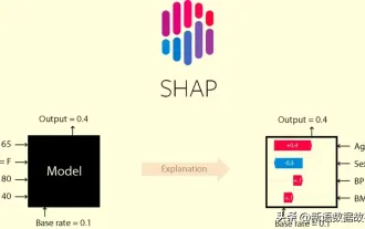 This article will take you to understand SHAP: model explanation for machine learning
Jun 01, 2024 am 10:58 AM
This article will take you to understand SHAP: model explanation for machine learning
Jun 01, 2024 am 10:58 AM
In the fields of machine learning and data science, model interpretability has always been a focus of researchers and practitioners. With the widespread application of complex models such as deep learning and ensemble methods, understanding the model's decision-making process has become particularly important. Explainable AI|XAI helps build trust and confidence in machine learning models by increasing the transparency of the model. Improving model transparency can be achieved through methods such as the widespread use of multiple complex models, as well as the decision-making processes used to explain the models. These methods include feature importance analysis, model prediction interval estimation, local interpretability algorithms, etc. Feature importance analysis can explain the decision-making process of a model by evaluating the degree of influence of the model on the input features. Model prediction interval estimate
 Implementing Machine Learning Algorithms in C++: Common Challenges and Solutions
Jun 03, 2024 pm 01:25 PM
Implementing Machine Learning Algorithms in C++: Common Challenges and Solutions
Jun 03, 2024 pm 01:25 PM
Common challenges faced by machine learning algorithms in C++ include memory management, multi-threading, performance optimization, and maintainability. Solutions include using smart pointers, modern threading libraries, SIMD instructions and third-party libraries, as well as following coding style guidelines and using automation tools. Practical cases show how to use the Eigen library to implement linear regression algorithms, effectively manage memory and use high-performance matrix operations.
 Five schools of machine learning you don't know about
Jun 05, 2024 pm 08:51 PM
Five schools of machine learning you don't know about
Jun 05, 2024 pm 08:51 PM
Machine learning is an important branch of artificial intelligence that gives computers the ability to learn from data and improve their capabilities without being explicitly programmed. Machine learning has a wide range of applications in various fields, from image recognition and natural language processing to recommendation systems and fraud detection, and it is changing the way we live. There are many different methods and theories in the field of machine learning, among which the five most influential methods are called the "Five Schools of Machine Learning". The five major schools are the symbolic school, the connectionist school, the evolutionary school, the Bayesian school and the analogy school. 1. Symbolism, also known as symbolism, emphasizes the use of symbols for logical reasoning and expression of knowledge. This school of thought believes that learning is a process of reverse deduction, through existing
 Is Flash Attention stable? Meta and Harvard found that their model weight deviations fluctuated by orders of magnitude
May 30, 2024 pm 01:24 PM
Is Flash Attention stable? Meta and Harvard found that their model weight deviations fluctuated by orders of magnitude
May 30, 2024 pm 01:24 PM
MetaFAIR teamed up with Harvard to provide a new research framework for optimizing the data bias generated when large-scale machine learning is performed. It is known that the training of large language models often takes months and uses hundreds or even thousands of GPUs. Taking the LLaMA270B model as an example, its training requires a total of 1,720,320 GPU hours. Training large models presents unique systemic challenges due to the scale and complexity of these workloads. Recently, many institutions have reported instability in the training process when training SOTA generative AI models. They usually appear in the form of loss spikes. For example, Google's PaLM model experienced up to 20 loss spikes during the training process. Numerical bias is the root cause of this training inaccuracy,
 Explainable AI: Explaining complex AI/ML models
Jun 03, 2024 pm 10:08 PM
Explainable AI: Explaining complex AI/ML models
Jun 03, 2024 pm 10:08 PM
Translator | Reviewed by Li Rui | Chonglou Artificial intelligence (AI) and machine learning (ML) models are becoming increasingly complex today, and the output produced by these models is a black box – unable to be explained to stakeholders. Explainable AI (XAI) aims to solve this problem by enabling stakeholders to understand how these models work, ensuring they understand how these models actually make decisions, and ensuring transparency in AI systems, Trust and accountability to address this issue. This article explores various explainable artificial intelligence (XAI) techniques to illustrate their underlying principles. Several reasons why explainable AI is crucial Trust and transparency: For AI systems to be widely accepted and trusted, users need to understand how decisions are made
 Improved detection algorithm: for target detection in high-resolution optical remote sensing images
Jun 06, 2024 pm 12:33 PM
Improved detection algorithm: for target detection in high-resolution optical remote sensing images
Jun 06, 2024 pm 12:33 PM
01 Outlook Summary Currently, it is difficult to achieve an appropriate balance between detection efficiency and detection results. We have developed an enhanced YOLOv5 algorithm for target detection in high-resolution optical remote sensing images, using multi-layer feature pyramids, multi-detection head strategies and hybrid attention modules to improve the effect of the target detection network in optical remote sensing images. According to the SIMD data set, the mAP of the new algorithm is 2.2% better than YOLOv5 and 8.48% better than YOLOX, achieving a better balance between detection results and speed. 02 Background & Motivation With the rapid development of remote sensing technology, high-resolution optical remote sensing images have been used to describe many objects on the earth’s surface, including aircraft, cars, buildings, etc. Object detection in the interpretation of remote sensing images
 Machine Learning in C++: A Guide to Implementing Common Machine Learning Algorithms in C++
Jun 03, 2024 pm 07:33 PM
Machine Learning in C++: A Guide to Implementing Common Machine Learning Algorithms in C++
Jun 03, 2024 pm 07:33 PM
In C++, the implementation of machine learning algorithms includes: Linear regression: used to predict continuous variables. The steps include loading data, calculating weights and biases, updating parameters and prediction. Logistic regression: used to predict discrete variables. The process is similar to linear regression, but uses the sigmoid function for prediction. Support Vector Machine: A powerful classification and regression algorithm that involves computing support vectors and predicting labels.
 Application of algorithms in the construction of 58 portrait platform
May 09, 2024 am 09:01 AM
Application of algorithms in the construction of 58 portrait platform
May 09, 2024 am 09:01 AM
1. Background of the Construction of 58 Portraits Platform First of all, I would like to share with you the background of the construction of the 58 Portrait Platform. 1. The traditional thinking of the traditional profiling platform is no longer enough. Building a user profiling platform relies on data warehouse modeling capabilities to integrate data from multiple business lines to build accurate user portraits; it also requires data mining to understand user behavior, interests and needs, and provide algorithms. side capabilities; finally, it also needs to have data platform capabilities to efficiently store, query and share user profile data and provide profile services. The main difference between a self-built business profiling platform and a middle-office profiling platform is that the self-built profiling platform serves a single business line and can be customized on demand; the mid-office platform serves multiple business lines, has complex modeling, and provides more general capabilities. 2.58 User portraits of the background of Zhongtai portrait construction
