K Nearest Neighbors Regression, Regression: Supervised Machine Learning

k-Nearest Neighbors Regression

k-Nearest Neighbors (k-NN) regression is a non-parametric method that predicts the output value based on the average (or weighted average) of the k-nearest training data points in the feature space. This approach can effectively model complex relationships in data without assuming a specific functional form.

The k-NN regression method can be summarized as follows:

1. Distance Metric: The algorithm uses a distance metric (commonly Euclidean distance) to determine the "closeness" of data points.
2. k Neighbors: The parameter k specifies how many nearest neighbors to consider when making predictions.
3. Prediction: The predicted value for a new data point is the average of the values of its k nearest neighbors.

Key Concepts

1. Non-Parametric: Unlike parametric models, k-NN does not assume a specific form for the underlying relationship between the input features and the target variable. This makes it flexible in capturing complex patterns.

2. Distance Calculation: The choice of distance metric can significantly affect the model's performance. Common metrics include Euclidean, Manhattan, and Minkowski distances.

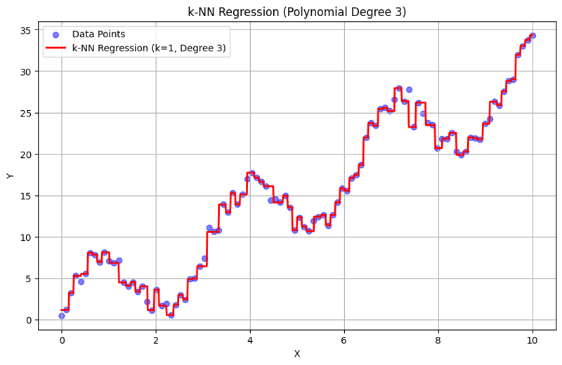
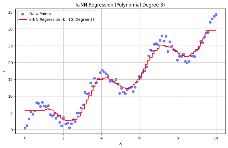
3. Choice of k: The number of neighbors (k) can be chosen based on cross-validation. A small k can lead to overfitting, while a large k can smooth out the prediction too much, potentially underfitting.

k-Nearest Neighbors Regression Example

This example demonstrates how to use k-NN regression with polynomial features to model complex relationships while leveraging the non-parametric nature of k-NN.

Python Code Example

1. Import Libraries

import numpy as np
import matplotlib.pyplot as plt
from sklearn.model_selection import train_test_split
from sklearn.preprocessing import PolynomialFeatures
from sklearn.neighbors import KNeighborsRegressor
from sklearn.metrics import mean_squared_error, r2_score

This block imports the necessary libraries for data manipulation, plotting, and machine learning.

2. Generate Sample Data

np.random.seed(42)  # For reproducibility
X = np.linspace(0, 10, 100).reshape(-1, 1)
y = 3 * X.ravel() + np.sin(2 * X.ravel()) * 5 + np.random.normal(0, 1, 100)

This block generates sample data representing a relationship with some noise, simulating real-world data variations.

3. Split the Dataset

X_train, X_test, y_train, y_test = train_test_split(X, y, test_size=0.2, random_state=42)

This block splits the dataset into training and testing sets for model evaluation.

4. Create Polynomial Features

degree = 3  # Change this value for different polynomial degrees
poly = PolynomialFeatures(degree=degree)
X_poly_train = poly.fit_transform(X_train)
X_poly_test = poly.transform(X_test)

This block generates polynomial features from the training and testing datasets, allowing the model to capture non-linear relationships.

5. Create and Train the k-NN Regression Model

k = 5  # Number of neighbors
knn_model = KNeighborsRegressor(n_neighbors=k)
knn_model.fit(X_poly_train, y_train)

This block initializes the k-NN regression model and trains it using the polynomial features derived from the training dataset.

6. Make Predictions

y_pred = knn_model.predict(X_poly_test)

This block uses the trained model to make predictions on the test set.

7. Plot the Results

plt.figure(figsize=(10, 6))
plt.scatter(X, y, color='blue', alpha=0.5, label='Data Points')
X_grid = np.linspace(0, 10, 1000).reshape(-1, 1)
X_poly_grid = poly.transform(X_grid)
y_grid = knn_model.predict(X_poly_grid)
plt.plot(X_grid, y_grid, color='red', linewidth=2, label=f'k-NN Regression (k={k}, Degree {degree})')
plt.title(f'k-NN Regression (Polynomial Degree {degree})')
plt.xlabel('X')
plt.ylabel('Y')
plt.legend()
plt.grid(True)
plt.show()

This block creates a scatter plot of the actual data points versus the predicted values from the k-NN regression model, visualizing the fitted curve.

Output with k = 1:

Output with k = 10:

This structured approach demonstrates how to implement and evaluate k-Nearest Neighbors regression with polynomial features. By capturing local patterns through averaging the responses of nearby neighbors, k-NN regression effectively models complex relationships in data while providing a straightforward implementation. The choice of k and polynomial degree significantly influences the model's performance and flexibility in capturing underlying trends.

The above is the detailed content of K Nearest Neighbors Regression, Regression: Supervised Machine Learning. For more information, please follow other related articles on the PHP Chinese website!