

Beating the Odds: The Mathematics Behind Casino Profits

Have you ever wondered why casinos always seem to win? In “Beating the Odds: The Mathematics Behind Casino Profits,” we’ll explore the simple math and clever strategies that ensure casinos make money in the long run. Through easy-to-understand examples and Monte Carlo simulations, we’ll reveal the secrets behind the house’s edge. Get ready to discover how casinos turn the odds in their favor!
Understanding the House Edge
The house edge is a fundamental concept in the world of casinos. It represents the average profit that the casino expects to make from each bet placed by players. Essentially, it is the percentage of each bet that the casino will retain in the long run.
The house edge exists because casinos do not pay out winning bets according to the “true odds” of the game. True odds represent the actual probability of an event occurring. By paying out at slightly lower odds, casinos ensure they make a profit over time.
The house edge (HE) is defined as the casino profit expressed as a percentage of the player’s original bet.
** European Roulette ** has only one green zero, giving it 37 numbers in total. If a player bets $1 on red, they have an 18/37 chance of winning $1 and a 19/37 chance of losing $1. The expected value is:
Expected Value=( 1 × 18/37 )+( −1 × 19/37 )= 18/37 − 19/37 = −1/37 ≈ −2.7%
Hence, In the European Roulette the house edge(HE) is around 2.7%.
Let’s make the game of our own to understand it more, A Simple Dice roll game.
import random

def roll_dice():
    roll = random.randint(1, 100)

    if roll == 100:
        print(roll, 'You rolled a 100 and lost. Better luck next time!')
        return False
    elif roll <= 50:
        print(roll, 'You rolled between 1 and 50 and lost.')
        return False
    else:
        print(roll, 'You rolled between 51 and 99 and won! Keep playing!')
        return True
In this game:
The player has a 1/100 chance of losing if the roll is 100.
The player has a 50/100 chance of losing if the roll is between 1 and 50.
The player has a 49/100 chance of winning if the roll is between 51 and 99.
Expected Value =(1× 49/100) + ( −1× 51/100) = 49/100 − 51/100 = −2/100 ≈ −2%
Therefore, the house edge is 2%.
Understanding Monte Carlo Simulation
Monte Carlo simulations are a powerful tool used to understand and predict complex systems by running numerous simulations of a process and observing the outcomes. In the context of casinos, Monte Carlo simulations can model various betting scenarios to show how the house edge ensures long-term profitability. Let’s explore how Monte Carlo simulations work and how they can be applied to a simple casino game.
What is a Monte Carlo Simulation?
A Monte Carlo simulation involves generating random variables to simulate a process multiple times and analyzing the results. By performing thousands or even millions of iterations, we can obtain a distribution of possible outcomes and gain insights into the likelihood of different events.
Applying Monte Carlo Simulation to the Dice Roll Game
We’ll use a Monte Carlo simulation to model the dice roll game we discussed earlier. This will help us understand how the house edge affects the game’s profitability over time.
`def monte_carlo_simulation(trials):
    wins = 0
    losses = 0

    for _ in range(trials):
        if roll_dice():
            wins += 1
        else:
            losses += 1

    win_percentage = (wins / trials) * 100
    loss_percentage = (losses / trials) * 100
    houseEdge= loss_percentage-win_percentage
    print(f"After {trials} trials:")
    print(f"Win percentage: {win_percentage:.2f}%")
    print(f"Loss percentage: {loss_percentage:.2f}%")
    print(f"House Edge: {houseEdge:.2f}%")

# Run the simulation with 10,000,000 trials
monte_carlo_simulation(10000000)`
Interpreting the Results
In this simulation, we run the dice roll game 10,000,000 times to observe the win and loss percentages. Given the house edge calculated earlier (2%), we expect the loss percentage to be slightly higher than the win percentage.
After running the simulation, you might see results like:
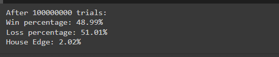
These results closely align with the theoretical probabilities (49% win, 51% loss), demonstrating how the house edge manifests over a large number of trials. The slight imbalance ensures the casino’s profitability in the long run.
Visualizing Short-Term Wins and Long-Term Losses
Monte Carlo simulations are powerful for modeling and predicting outcomes through repeated random sampling. In the context of gambling, we can use Monte Carlo simulations to understand the potential outcomes of different betting strategies.
We’ll simulate a single bettor who places the same initial wager in each round and observe how their account value evolves over a specified number of wagers.
Here’s how we can simulate and visualize the betting journey using Matplotlib:
def bettor_simulation(funds, initial_wager, wager_count):
    value = funds
    wager = initial_wager

    # Lists to store wager count and account value
    wX = []
    vY = []

    current_wager = 1

    while current_wager <= wager_count:
        if roll_dice():
            value += wager
        else:
            value -= wager

        wX.append(current_wager)
        vY.append(value)
        current_wager += 1

    return wX, vY

# Parameters for simulation
funds = 10000
initial_wager = 100
wager_count = 1000

# Run the simulation for a single bettor
wager_counts, account_values = bettor_simulation(funds, initial_wager, wager_count)

# Plotting the results
plt.figure(figsize=(12, 6))
plt.plot(wager_counts, account_values, label='Bettor 1', color='blue')
plt.xlabel('Wager Count')
plt.ylabel('Account Value')
plt.title('Betting Journey: Short-Term Wins vs Long-Term Losses')
plt.grid(True)
plt.legend()

# Highlighting the short-term and long-term trend
plt.axhline(y=funds, color='gray', linestyle='--', label='Initial Funds')
plt.axhline(y=account_values[0], color='green', linestyle='--', label='Starting Account Value')
plt.axhline(y=account_values[-1], color='red', linestyle='--', label='Final Account Value')

plt.legend()
plt.show()
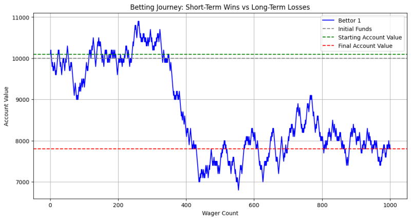
This graph illustrates how a bettor’s account value can fluctuate over time due to wins and losses. Initially, there may be periods of winning (green line above the starting value), but as the number of wagers increases, the cumulative effect of the house edge becomes evident. Eventually, the bettor’s account value tends to decline towards or below the initial funds (gray line), indicating long-term losses.
Conclusion
Understanding the mathematics behind casino profits reveals a clear advantage for the house in every game through the concept of the house edge. Despite occasional wins, the probability built into casino games ensures that most players will lose money over time. Monte Carlo simulations vividly illustrate these dynamics, showing how even short-term wins can mask long-term losses due to the casino’s statistical advantage. This insight into the mathematical certainty of casino profitability underscores the importance of informed decision-making and responsible gambling practices.
Next, we could explore additional visualizations or variations, such as comparing different betting strategies or analyzing the impact of varying initial wagers on the bettor’s outcomes.
Stay Connected:
GitHub: ezhillragesh
Twitter: ezhillragesh
Website: ragesh.me
Don’t hesitate to share your thoughts, ask questions, and contribute to the discussion.
Happy coding!
The above is the detailed content of Beating the Odds: The Mathematics Behind Casino Profits. For more information, please follow other related articles on the PHP Chinese website!

Hot AI Tools

Undresser.AI Undress
AI-powered app for creating realistic nude photos

AI Clothes Remover
Online AI tool for removing clothes from photos.

Undress AI Tool
Undress images for free

Clothoff.io
AI clothes remover

Video Face Swap
Swap faces in any video effortlessly with our completely free AI face swap tool!

Hot Article
Hot Tools

Notepad++7.3.1
Easy-to-use and free code editor

SublimeText3 Chinese version
Chinese version, very easy to use

Zend Studio 13.0.1
Powerful PHP integrated development environment

Dreamweaver CS6
Visual web development tools

SublimeText3 Mac version
God-level code editing software (SublimeText3)
Hot Topics
 1664
1664
 14
1422
52
1316
25
1266
29
1239
24
14
1422
52
1316
25
1266
29
1239
24

 Python vs. C : Applications and Use Cases Compared
Apr 12, 2025 am 12:01 AM
Python vs. C : Applications and Use Cases Compared
Apr 12, 2025 am 12:01 AM
Python is suitable for data science, web development and automation tasks, while C is suitable for system programming, game development and embedded systems. Python is known for its simplicity and powerful ecosystem, while C is known for its high performance and underlying control capabilities.
 The 2-Hour Python Plan: A Realistic Approach
Apr 11, 2025 am 12:04 AM
The 2-Hour Python Plan: A Realistic Approach
Apr 11, 2025 am 12:04 AM
You can learn basic programming concepts and skills of Python within 2 hours. 1. Learn variables and data types, 2. Master control flow (conditional statements and loops), 3. Understand the definition and use of functions, 4. Quickly get started with Python programming through simple examples and code snippets.
 Python: Games, GUIs, and More
Apr 13, 2025 am 12:14 AM
Python: Games, GUIs, and More
Apr 13, 2025 am 12:14 AM
Python excels in gaming and GUI development. 1) Game development uses Pygame, providing drawing, audio and other functions, which are suitable for creating 2D games. 2) GUI development can choose Tkinter or PyQt. Tkinter is simple and easy to use, PyQt has rich functions and is suitable for professional development.
 Python vs. C : Learning Curves and Ease of Use
Apr 19, 2025 am 12:20 AM
Python vs. C : Learning Curves and Ease of Use
Apr 19, 2025 am 12:20 AM
Python is easier to learn and use, while C is more powerful but complex. 1. Python syntax is concise and suitable for beginners. Dynamic typing and automatic memory management make it easy to use, but may cause runtime errors. 2.C provides low-level control and advanced features, suitable for high-performance applications, but has a high learning threshold and requires manual memory and type safety management.
 How Much Python Can You Learn in 2 Hours?
Apr 09, 2025 pm 04:33 PM
How Much Python Can You Learn in 2 Hours?
Apr 09, 2025 pm 04:33 PM
You can learn the basics of Python within two hours. 1. Learn variables and data types, 2. Master control structures such as if statements and loops, 3. Understand the definition and use of functions. These will help you start writing simple Python programs.
 Python and Time: Making the Most of Your Study Time
Apr 14, 2025 am 12:02 AM
Python and Time: Making the Most of Your Study Time
Apr 14, 2025 am 12:02 AM
To maximize the efficiency of learning Python in a limited time, you can use Python's datetime, time, and schedule modules. 1. The datetime module is used to record and plan learning time. 2. The time module helps to set study and rest time. 3. The schedule module automatically arranges weekly learning tasks.
 Python: Exploring Its Primary Applications
Apr 10, 2025 am 09:41 AM
Python: Exploring Its Primary Applications
Apr 10, 2025 am 09:41 AM
Python is widely used in the fields of web development, data science, machine learning, automation and scripting. 1) In web development, Django and Flask frameworks simplify the development process. 2) In the fields of data science and machine learning, NumPy, Pandas, Scikit-learn and TensorFlow libraries provide strong support. 3) In terms of automation and scripting, Python is suitable for tasks such as automated testing and system management.
 Python: Automation, Scripting, and Task Management
Apr 16, 2025 am 12:14 AM
Python: Automation, Scripting, and Task Management
Apr 16, 2025 am 12:14 AM
Python excels in automation, scripting, and task management. 1) Automation: File backup is realized through standard libraries such as os and shutil. 2) Script writing: Use the psutil library to monitor system resources. 3) Task management: Use the schedule library to schedule tasks. Python's ease of use and rich library support makes it the preferred tool in these areas.
