Classification is a supervised learning technique used in machine learning and data science to categorize data into predefined classes or labels. It involves training a model to assign input data points to one of several discrete categories based on their features. The main purpose of classification is to accurately predict the class or category of new, unseen data points.
1. Binary Classification
2. Multiclass Classification
Linear classifiers are a category of classification algorithms that use a linear decision boundary to separate different classes in the feature space. They make predictions by combining the input features through a linear equation, typically representing the relationship between the features and the target class labels. The main purpose of linear classifiers is to efficiently classify data points by finding a hyperplane that divides the feature space into distinct classes.
Logistic Regression is a statistical method used for binary classification tasks in machine learning and data science. It is a part of linear classifiers and differs from linear regression by predicting the probability of occurrence of an event through fitting data to a logistic curve.
1. Logistic Function (Sigmoid Function)
2. Logistic Regression Equation
MLE is used to estimate the parameters (coefficients) of the logistic regression model by maximizing the likelihood of observing the data given the model.
Equation: Maximizing the log-likelihood function involves finding the parameters that maximize the probability of observing the data.
The cost function in logistic regression measures the difference between predicted probabilities and actual class labels. The goal is to minimize this function to improve the model's predictive accuracy.
Log Loss (Binary Cross-Entropy):
The log loss function is commonly used in logistic regression for binary classification tasks.
Log Loss = -(1/n) * Σ [y * log(ŷ) + (1 - y) * log(1 - ŷ)]
where:
The log loss penalizes predictions that are far from the actual class label, encouraging the model to produce accurate probabilities.
Loss minimization in logistic regression involves finding the values of the model parameters that minimize the cost function value. This process is also known as optimization. The most common method for loss minimization in logistic regression is the Gradient Descent algorithm.
Gradient Descent is an iterative optimization algorithm used to minimize the cost function in logistic regression. It adjusts the model parameters in the direction of the steepest descent of the cost function.
Steps of Gradient Descent:
Initialize Parameters: Start with initial values for the model parameters (e.g., coefficients w0, w1, ..., wn).
Calculate Gradient: Compute the gradient of the cost function with respect to each parameter. The gradient is the partial derivative of the cost function.
Update Parameters: Adjust the parameters in the opposite direction of the gradient. The adjustment is controlled by the learning rate (α), which determines the size of the steps taken towards the minimum.
Repeat: Iterate the process until the cost function converges to a minimum value (or a pre-defined number of iterations is reached).
Parameter Update Rule:
For each parameter wj:
wj = wj - α * (∂/∂wj) Log Loss
where:
The partial derivative of the log loss with respect to wj can be calculated as:
(∂/∂wj) Log Loss = -(1/n) * Σ [ (yi - ŷi) * xij / (ŷi * (1 - ŷi)) ]
where:
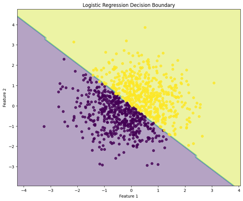
Logistic regression is a technique used for binary classification tasks, modeling the probability that a given input belongs to a particular class. This example demonstrates how to implement logistic regression using synthetic data, evaluate the model's performance, and visualize the decision boundary.
1. Import Libraries
import numpy as np
import matplotlib.pyplot as plt
from sklearn.model_selection import train_test_split
from sklearn.linear_model import LogisticRegression
from sklearn.metrics import accuracy_score, confusion_matrix, classification_report
This block imports the necessary libraries for data manipulation, plotting, and machine learning.
2. Generate Sample Data
np.random.seed(42)  # For reproducibility
X = np.random.randn(1000, 2)
y = (X[:, 0] + X[:, 1] > 0).astype(int)
This block generates sample data with two features, where the target variable y is defined based on whether the sum of the features is greater than zero, simulating a binary classification scenario.
3. Split the Dataset
X_train, X_test, y_train, y_test = train_test_split(X, y, test_size=0.2, random_state=42)
This block splits the dataset into training and testing sets for model evaluation.
4. Create and Train the Logistic Regression Model
model = LogisticRegression(random_state=42)
model.fit(X_train, y_train)
This block initializes the logistic regression model and trains it using the training dataset.
5. Make Predictions
y_pred = model.predict(X_test)
This block uses the trained model to make predictions on the test set.
6. Evaluate the Model
accuracy = accuracy_score(y_test, y_pred)
conf_matrix = confusion_matrix(y_test, y_pred)
class_report = classification_report(y_test, y_pred)

print(f"Accuracy: {accuracy:.4f}")
print("\nConfusion Matrix:")
print(conf_matrix)
print("\nClassification Report:")
print(class_report)
Output:
Accuracy: 0.9950

Confusion Matrix:
[[ 92   0]
 [  1 107]]

Classification Report:
              precision    recall  f1-score   support

           0       0.99      1.00      0.99        92
           1       1.00      0.99      1.00       108

    accuracy                           0.99       200
   macro avg       0.99      1.00      0.99       200
weighted avg       1.00      0.99      1.00       200
This block calculates and prints the accuracy, confusion matrix, and classification report, providing insights into the model's performance.
7. Visualize the Decision Boundary
x_min, x_max = X[:, 0].min() - 1, X[:, 0].max() + 1
y_min, y_max = X[:, 1].min() - 1, X[:, 1].max() + 1
xx, yy = np.meshgrid(np.arange(x_min, x_max, 0.1),
                     np.arange(y_min, y_max, 0.1))
Z = model.predict(np.c_[xx.ravel(), yy.ravel()])
Z = Z.reshape(xx.shape)

plt.figure(figsize=(10, 8))
plt.contourf(xx, yy, Z, alpha=0.4)
plt.scatter(X[:, 0], X[:, 1], c=y, alpha=0.8)
plt.xlabel("Feature 1")
plt.ylabel("Feature 2")
plt.title("Logistic Regression Decision Boundary")
plt.show()
This block visualizes the decision boundary created by the logistic regression model, illustrating how the model separates the two classes in the feature space.
Output:

This structured approach demonstrates how to implement and evaluate logistic regression, providing a clear understanding of its capabilities for binary classification tasks. The visualization of the decision boundary aids in interpreting the model's predictions.
Logistic regression can also be applied to multiclass classification tasks. This example demonstrates how to implement logistic regression using synthetic data, evaluate the model's performance, and visualize the decision boundary for three classes.
1. Import Libraries
import numpy as np
import matplotlib.pyplot as plt
from sklearn.model_selection import train_test_split
from sklearn.linear_model import LogisticRegression
from sklearn.metrics import accuracy_score, confusion_matrix, classification_report
This block imports the necessary libraries for data manipulation, plotting, and machine learning.
2. Generate Sample Data with 3 Classes
np.random.seed(42)  # For reproducibility
n_samples = 999  # Total number of samples
n_samples_per_class = 333  # Ensure this is exactly n_samples // 3

# Class 0: Top-left corner
X0 = np.random.randn(n_samples_per_class, 2) * 0.5 + [-2, 2]

# Class 1: Top-right corner
X1 = np.random.randn(n_samples_per_class, 2) * 0.5 + [2, 2]

# Class 2: Bottom center
X2 = np.random.randn(n_samples_per_class, 2) * 0.5 + [0, -2]

# Combine the data
X = np.vstack([X0, X1, X2])
y = np.hstack([np.zeros(n_samples_per_class),
               np.ones(n_samples_per_class),
               np.full(n_samples_per_class, 2)])

# Shuffle the dataset
shuffle_idx = np.random.permutation(n_samples)
X, y = X[shuffle_idx], y[shuffle_idx]
This block generates synthetic data for three classes located in different regions of the feature space.
3. Split the Dataset
X_train, X_test, y_train, y_test = train_test_split(X, y, test_size=0.2, random_state=42)
This block splits the dataset into training and testing sets for model evaluation.
4. Create and Train the Logistic Regression Model
model = LogisticRegression(random_state=42)
model.fit(X_train, y_train)
This block initializes the logistic regression model and trains it using the training dataset.
5. Make Predictions
y_pred = model.predict(X_test)
This block uses the trained model to make predictions on the test set.
6. Evaluate the Model
accuracy = accuracy_score(y_test, y_pred)
conf_matrix = confusion_matrix(y_test, y_pred)
class_report = classification_report(y_test, y_pred)

print(f"Accuracy: {accuracy:.4f}")
print("\nConfusion Matrix:")
print(conf_matrix)
print("\nClassification Report:")
print(class_report)
Output:
Accuracy: 1.0000

Confusion Matrix:
[[54  0  0]
 [ 0 65  0]
 [ 0  0 81]]

Classification Report:
              precision    recall  f1-score   support

         0.0       1.00      1.00      1.00        54
         1.0       1.00      1.00      1.00        65
         2.0       1.00      1.00      1.00        81

    accuracy                           1.00       200
   macro avg       1.00      1.00      1.00       200
weighted avg       1.00      1.00      1.00       200
This block calculates and prints the accuracy, confusion matrix, and classification report, providing insights into the model's performance.
7. Visualize the Decision Boundary
x_min, x_max = X[:, 0].min() - 1, X[:, 0].max() + 1
y_min, y_max = X[:, 1].min() - 1, X[:, 1].max() + 1
xx, yy = np.meshgrid(np.arange(x_min, x_max, 0.1),
                     np.arange(y_min, y_max, 0.1))
Z = model.predict(np.c_[xx.ravel(), yy.ravel()])
Z = Z.reshape(xx.shape)

plt.figure(figsize=(10, 8))
plt.contourf(xx, yy, Z, alpha=0.4, cmap='RdYlBu')
scatter = plt.scatter(X[:, 0], X[:, 1], c=y, cmap='RdYlBu', edgecolor='black')
plt.xlabel("Feature 1")
plt.ylabel("Feature 2")
plt.title("Multiclass Logistic Regression Decision Boundary")
plt.colorbar(scatter)
plt.show()
This block visualizes the decision boundaries created by the logistic regression model, illustrating how the model separates the three classes in the feature space.
Output:

This structured approach demonstrates how to implement and evaluate logistic regression for multiclass classification tasks, providing a clear understanding of its capabilities and the effectiveness of visualizing decision boundaries.
Evaluating a logistic regression model involves assessing its performance in predicting binary or multiclass outcomes. Below are key methods for evaluation:
  from sklearn.metrics import accuracy_score

  accuracy = accuracy_score(y_test, y_pred)
  print(f'Accuracy: {accuracy:.4f}')
  from sklearn.metrics import confusion_matrix

  conf_matrix = confusion_matrix(y_test, y_pred)
  print("\nConfusion Matrix:")
  print(conf_matrix)
  from sklearn.metrics import precision_score

  precision = precision_score(y_test, y_pred, average='weighted')
  print(f'Precision: {precision:.4f}')
  from sklearn.metrics import recall_score

  recall = recall_score(y_test, y_pred, average='weighted')
  print(f'Recall: {recall:.4f}')
  from sklearn.metrics import f1_score

  f1 = f1_score(y_test, y_pred, average='weighted')
  print(f'F1 Score: {f1:.4f}')
Cross-validation techniques provide a more reliable evaluation of model performance by assessing it across different subsets of the dataset.
  from sklearn.model_selection import KFold, cross_val_score

  kf = KFold(n_splits=5, shuffle=True, random_state=42)
  scores = cross_val_score(model, X, y, cv=kf, scoring='accuracy')
  print(f'Cross-Validation Accuracy: {np.mean(scores):.4f}')
  from sklearn.model_selection import StratifiedKFold

  skf = StratifiedKFold(n_splits=5)
  scores = cross_val_score(model, X, y, cv=skf, scoring='accuracy')
  print(f'Stratified K-Fold Cross-Validation Accuracy: {np.mean(scores):.4f}')
By utilizing these evaluation methods and cross-validation techniques, practitioners can gain insights into the effectiveness of their logistic regression model and its ability to generalize to unseen data.
Regularization helps mitigate overfitting in logistic regression by adding a penalty term to the loss function, encouraging simpler models. The two primary forms of regularization in logistic regression are L1 regularization (Lasso) and L2 regularization (Ridge).
Concept: L2 regularization adds a penalty equal to the square of the magnitude of coefficients to the loss function.
Loss Function: The modified loss function for Ridge logistic regression is expressed as:
Loss = -Σ[yi * log(ŷi) + (1 - yi) * log(1 - ŷi)] + λ * Σ(wj^2)
Where:
Effects:
Concept: L1 regularization adds a penalty equal to the absolute value of the magnitude of coefficients to the loss function.
Loss Function: The modified loss function for Lasso logistic regression can be expressed as:
Loss = -Σ[yi * log(ŷi) + (1 - yi) * log(1 - ŷi)] + λ * Σ|wj|
Where:
Effects:
By applying regularization techniques in logistic regression, practitioners can enhance model generalization and manage the bias-variance tradeoff effectively.
The above is the detailed content of Logistic Regression, Classification: Supervised Machine Learning. For more information, please follow other related articles on the PHP Chinese website!
 Why is my phone not turned off but when someone calls me it prompts me to turn it off?
 How to set up hibernation in Win7 system
 What does Jingdong plus mean?
 The difference between cellpadding and cellspacing
 Sublime input Chinese method
 How to solve garbled characters in PHP
 What currency is USDT?
 rtmp server
 What is digital currency


