Solve complex financial calculations with 3 Excel financial functions

Original title: "These 3 Excel financial functions are undervalued again!" 》

The author of this article: Xiaohua

The editor of this article: Yanlan

Recently, Xiaohua encountered an interesting question, which came from the soul of an old friend:

How to pay monthly annuity and private mutual insurance finance make a choice?

The basic information of these two financial products is as follows:

Monthly annuity:

Pay 1,000 yuan per month, annualized interest rate is 3%, 2-year term, and the principal and interest can be withdrawn in one go at maturity.

Mutual Insurance Finance:

Pay the principal of 1,000 yuan every month, and the monthly principal will be calculated at 10% interest, with a 2-year term. There are 24 people participating in the same product. Every month, one person must receive all the principal and interest paid by others. The next month after receiving the payment, one person must pay an interest of 100 yuan/month.

How to compare the pros and cons of these two financial products?

We can consider this issue from the terminal value method, rate of return method and IRR method, and by the way share with you some usage of financial functions.

1. Terminal value method

The terminal value analysis method is to calculate the final value of the net benefit of the plan (project) after determining the base year, conversion interest rate, and cash flow. The higher the terminal value, the greater the economic feasibility of the solution.

How much principal and interest can be received after the equal-amount annuity matures? This problem can be calculated using the final value function FV.

Annuity future value formula:

=-FV(B3/12,C3,A3)

It can be seen that if an annuity of 1,000 yuan is paid every month, the interest rate is calculated at 3%. After 2 years, a total of 24,703 yuan in principal and interest will be received.

The final value of "Mutual Insurance Finance" (assuming no rolling investment) is related to the order in which the principal and interest are withdrawn. The later the withdrawal, the greater the income. The final value is calculated as follows:

=S2*U2+S2*T2*(V2-1)-S2*T2*(U2-V2)

From the perspective of the final value method, if you can ensure the receipt When the payment period is after 16 periods, the income of "Mutual Insurance Finance" is greater than the monthly annuity. When the receiving period is earlier than 16 periods, the income of "Mutual Insurance Finance" is less than the monthly annuity.

The terminal value method is suitable for investment plans with a comparable investment scale.

2. Rate of Return Method

When I told this preliminary conclusion to my old friend, he asked in disbelief:

Why is the nominal interest rate of "Mutual Insurance Finance" 10%? But only 1/3 of the participants’ income is higher than that of monthly annuity, which has a return rate of only 3%?

This involves the calculation of profitability.

The rate of return method is an investment decision-making method that compares the average annual net rate of return of an investment project with the capital cost of the investment to determine whether the investment is desirable, and then selects the investment plan with the highest rate of return among the available investment plans. .

Obviously, the monthly annuity yield is consistent with the nominal interest rate, which is 3%.

So, what is the return rate for each payment period of "Mutual Insurance Finance"?

We can use the RATE function to calculate.

The rate of return of "Mutual Insurance Finance" is calculated as follows:

=RATE(U2-S2,0,W2,0)*12

From the rate of return method, although The nominal interest rate of "Mutual Insurance Finance" is as high as 10%, but in fact, only when participants receive principal and interest after 16 periods, the rate of return can reach 3%. If received before then, the rate of return is lower than the income of monthly annuity. The rate is 3%. It can be seen that the yield rate of "mutual insurance finance" is still high.

However, it is unfair to evaluate that the income of "Mutual Insurance Finance" is not as good as that of monthly annuity. The reason is that the principal and interest of monthly annuity cannot be recovered until it matures, while "Mutual Insurance Finance" may realize capital inflow in advance. If this part Funds will be used for investment again, and "mutual insurance finance" will be greatly improved.

In financial management, time value is often used to explain this difference. The internal rate of return (IRR) and net present value (NPV) can be used to measure the dynamic return of an investment.

Below, we choose NPV to compare these two financial products. The IRR comparison method is not applicable to this case.

3. Net present value method

Before calculating the net present value, we need to list the cash flows of the two products in each period, and then use the NPV function to calculate.

毎月1,000元の年金を24回支払うと、24,703元が一括で回収されます。キャッシュフローとNPVは次のように計算されます。

=NPV(B3) /12,B2:Y2)

ここでは、毎月の年金の金利が割引率として直接選択され、その正味現在価値は 0 になるはずです。 「相互保険金融」の正味現在価値を計算する際には、引き続きこの割引率を使用します。後者の正味現在価値が 0 より大きい場合は、後者の投資収益が優れていることを意味し、それ以外の場合は後者の方が悪いことを意味します。

「相互保険ファイナンス」には複数の引き出し期間があるため、この商品のIRRを計算する際には、それを実現するためのシミュレーションテーブルを使用する必要があります。

「共済金融」NPV計算:

❶ 脱退期間を変数として、変数に基づいて計算された各期間のキャッシュフローをリスト化します。

元本のキャッシュフロー。正の数値は支払いを示し、負の数値は引き出しを示します。

=IF(E$4=$G$2,-$D$2*23,$D$2)

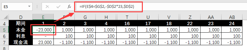
利息のキャッシュフロー。正の数値は支払いを示し、負の数値は受け取りを示します。

=IFS(E4$G$2,$D$2*$E$2)

連結キャッシュフロー:

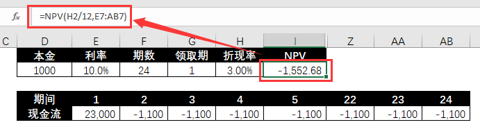
❷ 単一引き出し期間でのIRRを計算します。

=NPV(H2/12,E7:AB7)

❸ シミュレーションテーブルを使用して、さまざまな抽出期間に対応するNPVを計算します。

① 必要な収集期間変数値をリストし、最初の行に対応する結果値をリンクします。

② リンク行、変数値領域、結果値領域を選択し、以下の手順に従ってシミュレーション操作を完了します。

シミュレーション計算結果は以下の通りです。

NPVの観点から見ると、「共済財政」と毎月の年金収入は同等です。

前者のすべての参加者の中で、相対的な収益はまちまちです。これは、より早い請求期間を持つ参加者は、高金利の損失をある程度回避できるローリング投資の方がより早くキャッ​​シュインを獲得できるためです。

まとめると、ローリング投資の実現や確実性の追求が不可能な場合には、安定した運用収益とより高い平均静的収益が得られるこの商品を選択する必要があります。

より高い動的収益を追求する場合、または元本と利息を引き出した後に二次投資を行うことができる場合、財務管理には「相互保険ファイナンス」を選択する必要があります。後者には、より高い正味現在価値と静的収益を達成する機会があります。

上記は、金融商品選択問題からの Xiaohua の拡張であり、以下を含むいくつかの Excel 財務公式と関数の使用法を説明しています。あなたが財務会計士である場合、または財務計算が必要な場合や財務計算に興味がある場合は、これらの公式と実際の事例が役立つでしょう。

Xiaohua は今後も Excel の金融収入計算の他の実践例を共有し、数式やツールの使用方法を理解できるよう実践的な経験を活用していきますので、ご期待ください。

The above is the detailed content of Solve complex financial calculations with 3 Excel financial functions. For more information, please follow other related articles on the PHP Chinese website!