Excel tables are software that many users use in their daily work. Various data are filled in the tables. Many users want to draw charts to display data, but don’t know how to make them. To address this problem, today’s software In this tutorial, users will share two solutions. Let’s take a look at the detailed steps.

Excel data chart tutorial
Question: How to generate a function graph simply and quickly? Brief explanation: A function diagram is a diagram that visualizes function call relationships and can help you understand the structure and dependencies of your code. Continue reading: PHP editor Youzi will introduce you to a simple and practical method, using a free tool to generate function diagrams, allowing you to easily master the code flow.

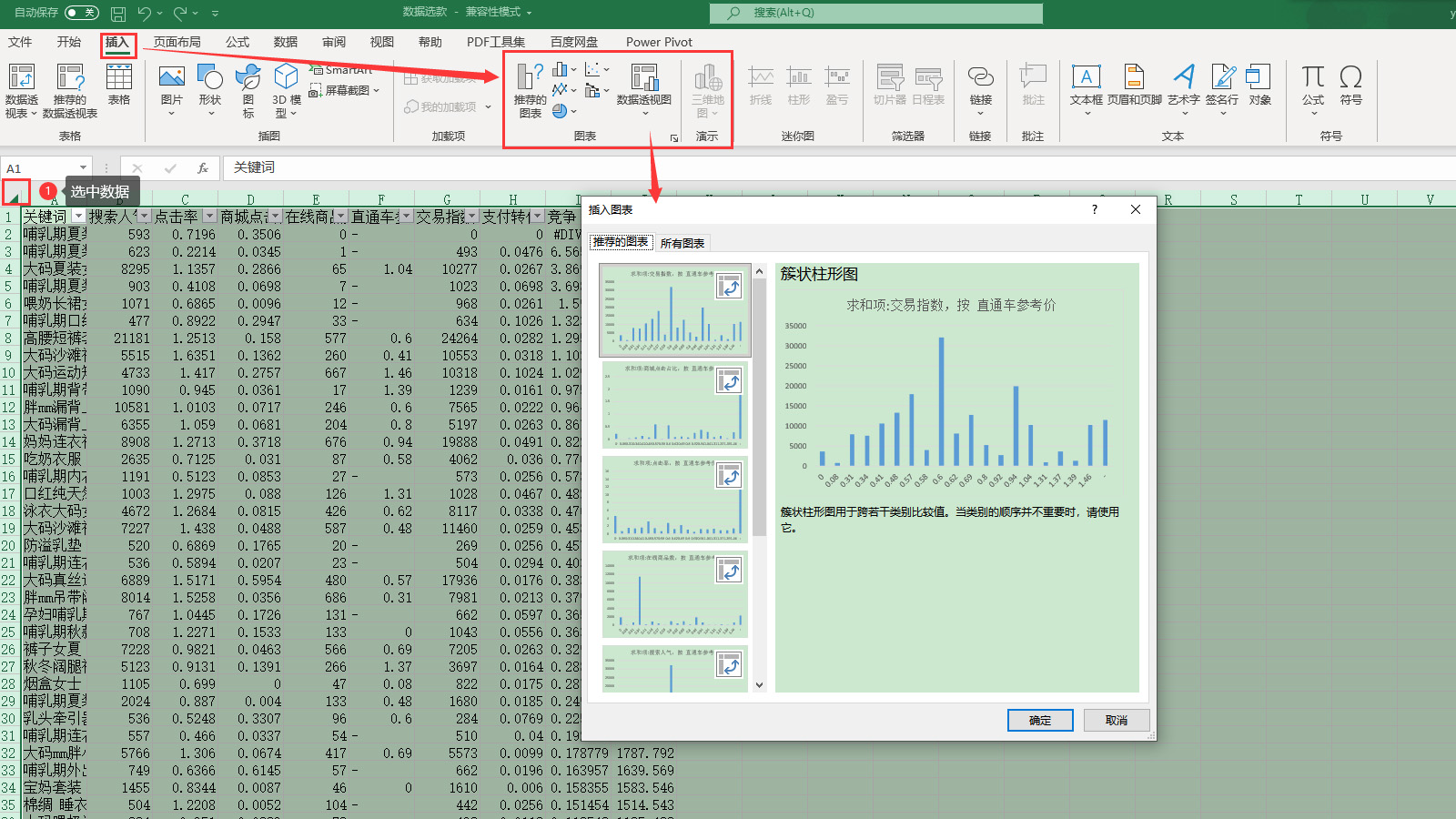
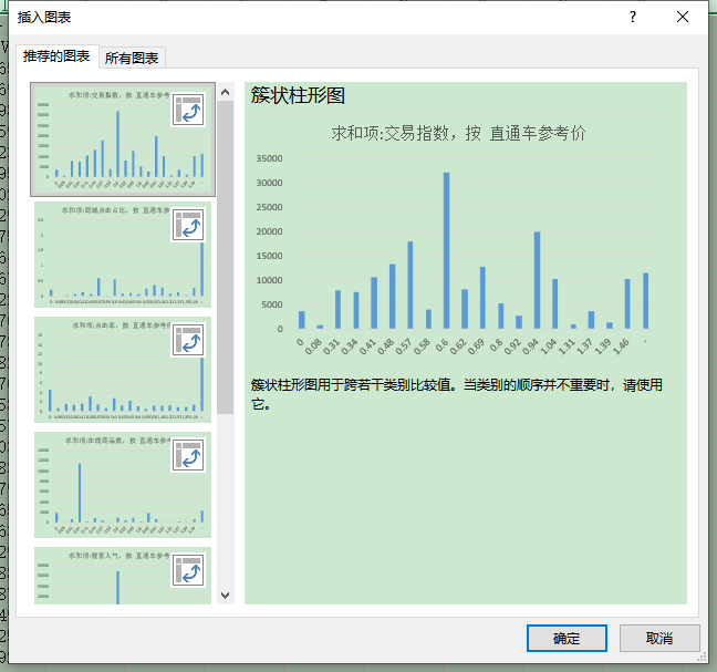
Open the data through Microsoft 365 Excel, then select all the data, click Insert on the top menu bar, find the chart area on the toolbar, and click Recommended Charts. Open the settings window (Figure 2).

First, we can directly select the recommended icon on the left, preview the rendering on the right, and click OK to insert it into the table.
In addition to the column chart like the step in Figure 2, there are many function charts. Let’s take a look at how to switch.
2. Edit and modify function graph
1. Add function graph

When modifying other graphics, click all charts in the chart setting box and select according to the graphic style. As shown in Figure 3, we select one of the stitch removal diagrams and click OK to insert it into the chart (Figure 4).

The function graph is ready. Microsoft 365 also marks different data with lines of different colors. According to the trend, you can quickly find the data you want. Click the function chart to generate touch points around it. Drag the touch points to zoom in or out of the chart.
2. Modify the title

Select the title in the icon and enter text directly, such as a selection chart. In addition to modifying the text content of the chart, we can also modify the style of the title. Double-click the title, and the chart title formatting area will appear on the right side of Excel. In this area, we can edit the text color, transparency, etc. of the title (Figure 6).

In addition to designing the text style, you can also set the alignment of the title. Click to select the title, click Title Options, and in the size and attribute settings area, you can edit the direction and vertical alignment of the text (Figure 7).

3. Modify the coordinate axis

Click the left coordinate axis of the selected icon, Set the axis format position on the right to edit the axis options. The coordinate axis option defaults to automatic, that is, the software will automatically establish the corresponding coordinate axis value based on the data. If you need to adjust, just double-click the input box and edit the value.
The above is the detailed content of How to draw data charts in Excel Excel data chart drawing tutorial. For more information, please follow other related articles on the PHP Chinese website!


