
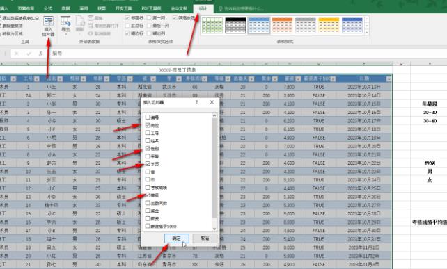
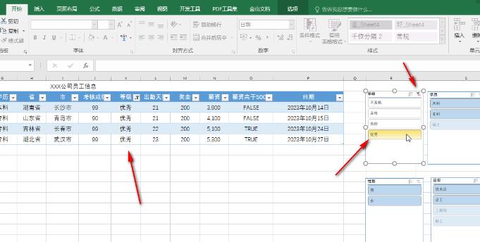
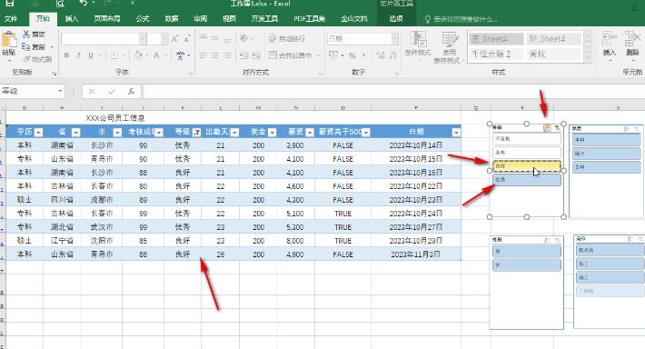
Excel spreadsheet is a very easy-to-use office software with rich and powerful functions. If you want to insert a slicer into an Excel table to facilitate filtering data, how do you do it? In fact, the operation method is very simple, just a few very simple steps are enough. Next, the editor will introduce the method. Setting method 1. Double-click to open the Excel table to enter the editing interface, select the data area (only select the header and the content below, do not select the title), press Ctrl+T, or click the Apply Table Format button in the Home tab and select a desired format.


The above is the detailed content of How to insert and filter using slicers in Excel. For more information, please follow other related articles on the PHP Chinese website!


