Finding Shortest Paths

The shortest path between two vertices is a path with the minimum total weights.
Given a graph with nonnegative weights on the edges, a well-known algorithm for finding a shortest path between two vertices was discovered by Edsger Dijkstra, a Dutch computer scientist. In order to find a shortest path from vertex s to vertex v, Dijkstra’s algorithm finds the shortest path from s to all vertices. So Dijkstra’s algorithm is known as a single-source shortest path algorithm. The algorithm uses cost[v] to store the cost of a shortest path from vertex v to the source vertex s. cost[s] is 0. Initially assign infinity to cost[v] for all other vertices. The algorithm repeatedly finds a vertex u in V – T with the smallest cost[u] and moves u to T.

The algorithm is described in code below.

Input: a graph G = (V, E) with non-negative weights
Output: a shortest path tree with the source vertex s as the root
 1 ShortestPathTree getShortestPath(s) {
 2 Let T be a set that contains the vertices whose
 3 paths to s are known; Initially T is empty;
 4 Set cost[s] = 0; and cost[v] = infinity for all other vertices in V;
 5
 6 while (size of T < n) {
 7 Find u not in T with the smallest cost[u];
 8 Add u to T;
 9 for (each v not in T and (u, v) in E)
10 if (cost[v] > cost[u] + w(u, v)) {
11 cost[v] = cost[u] + w(u, v); parent[v] = u;
12 }
13 }
14 }

This algorithm is very similar to Prim’s for finding a minimum spanning tree. Both algorithms divide the vertices into two sets: T and V - T. In the case of Prim’s algorithm, set T contains the vertices that are already added to the tree. In the case of Dijkstra’s, set T contains the vertices whose shortest paths to the source have been found. Both algorithms repeatedly find a vertex from V – T and add it to T. In the case of Prim’s algorithm, the vertex is adjacent to some vertex in the set with the minimum weight on the edge. In Dijkstra’s algorithm, the vertex is adjacent to some vertex in the set with the minimum total cost to the source.

The algorithm starts by setting cost[s] to 0 (line 4), sets cost[v] to infinity for all other vertices. It then continuously adds a vertex (say u) from V – T into T with smallest cost[u] (lines 7–8), as shown in Figure below a. After adding u to T, the algorithm updates cost[v] and parent[v] for each v not in T if (u, v) is in T and cost[v] > cost[u] + w(u, v) (lines 10–11).

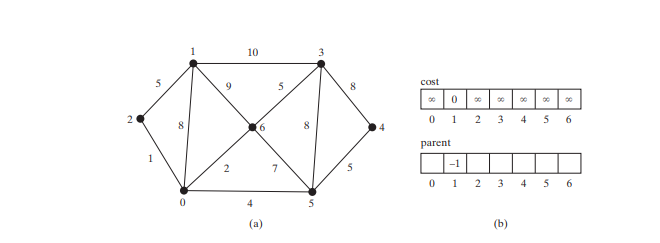
Let us illustrate Dijkstra’s algorithm using the graph in Figure below a. Suppose the source vertex is 1. Therefore, cost[1] = 0 and the costs for all other vertices are initially ∞, as shown in Figure below b. We use the parent[i] to denote the parent of i in the path. For convenience, set the parent of the source node to -1.

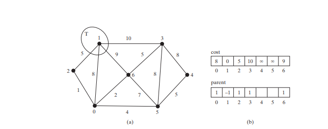
Initially set T is empty. The algorithm selects the vertex with the smallest cost. In this case, the vertex is 1. The algorithm adds 1 to T, as shown in Figure below a. Afterwards, it adjusts the cost for each vertex adjacent to 1. The cost for vertices 2, 0, 6, and 3 and their parents are now updated, as shown, as shown in Figure below b.

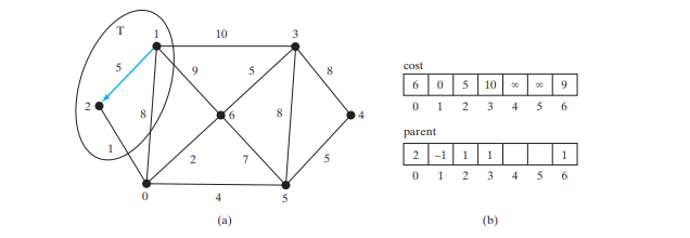
Vertices 2, 0, 6, and 3 are adjacent to the source vertex, and vertex 2 is the one in V-T with the smallest cost, so add 2 to T, as shown in Figure below and update the cost and parent for vertices in V-T and adjacent to 2. cost[0] is now updated to 6 and its parent is set to 2. The arrow line from 1 to 2 indicates that 1 is the parent of 2 after 2 is added into T.

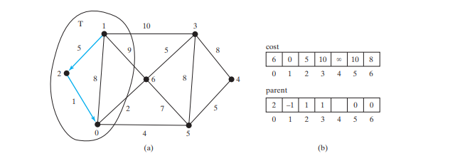
Now T contains {1, 2}. Vertex 0 is the one in V-T with the smallest cost, so add 0 to T, as shown in Figure below and update the cost and parent for vertices in V-T and adjacent to 0 if applicable. cost[5] is now updated to 10 and its parent is set to 0 and cost[6] is now updated to 8 and its parent is set to 0.

Now T contains {1, 2, 0}. Vertex 6 is the one in V-T with the smallest cost, so add 6 to T, as shown in Figure below and update the cost and parent for vertices in V-T and adjacent to 6 if applicable.

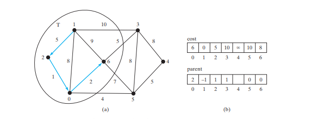
Now T contains {1, 2, 0, 6}. Vertex 3 or 5 is is the one in V-T with the smallest cost. You may add either 3 or 5 into T. Let us add 3 to T, as shown in Figure below and update the cost and parent for vertices in V-T and adjacent to 3 if applicable. cost[4] is now updated to 18 and its parent is set to 3.

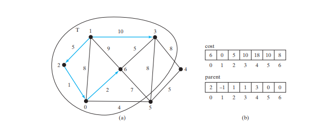
Now T contains {1, 2, 0, 6, 3}. Vertex 5 is the one in V-T with the smallest cost, so add 5 to T, as shown in Figure below and update the cost and parent for vertices in V-T and adjacent to 5 if applicable. cost[4] is now updated to 10 and its parent is set to 5.

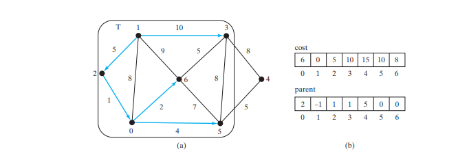
Now T contains {1, 2, 0, 6, 3, 5}. Vertex 4 is the one in V-T with the smallest cost, so add 4 to T, as shown in Figure below.

As you can see, the algorithm essentially finds all shortest paths from a source vertex, which produces a tree rooted at the source vertex. We call this tree a single-source all-shortest-path tree (or simply a shortest-path tree). To model this tree, define a class named ShortestPathTree that extends the Tree class, as shown in Figure below. ShortestPathTree is defined as an inner class in WeightedGraph in lines 200–224 in WeightedGraph.java.

The getShortestPath(int sourceVertex) method was implemented in lines 156–197 in WeightedGraph.java. The method sets cost[sourceVertex] to 0 (line 162) and cost[v] to infinity for all other vertices (lines 159–161). The parent of sourceVertex is set to -1 (line 166). T is a list that stores the vertices added into the shortest path tree (line 169). We use a list for T rather than a set in order to record the order of the vertices added to T.

Initially, T is empty. To expand T, the method performs the following operations:

1. Find the vertex u with the smallest cost[u] (lines 175–181) and add it into T (line 183).
2. After adding u in T, update cost[v] and parent[v] for each v adjacent to u in V-T if cost[v] > cost[u] + w(u, v) (lines 186–192).

Once all vertices from s are added to T, an instance of ShortestPathTree is created (line 196).

The ShortestPathTree class extends the Tree class (line 200). To create an instance of ShortestPathTree, pass sourceVertex, parent, T, and cost (lines 204–205). sourceVertex becomes the root in the tree. The data fields root, parent, and searchOrder are defined in the Tree class, which is an inner class defined in AbstractGraph.

Note that testing whether a vertex i is in T by invoking T.contains(i) takes O(n) time, since T is a list. Therefore, the overall time complexity for this implemention is O(n^3).

Dijkstra’s algorithm is a combination of a greedy algorithm and dynamic programming. It is a greedy algorithm in the sense that it always adds a new vertex that has the shortest distance to the source. It stores the shortest distance of each known vertex to the source and uses it later to avoid redundant computing, so Dijkstra’s algorithm also uses dynamic programming.

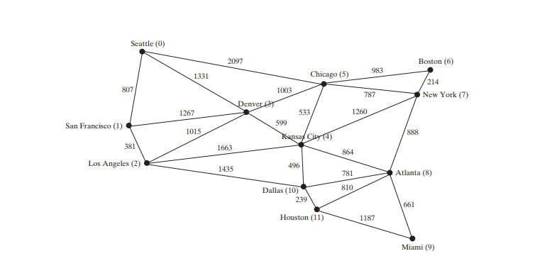
The code below gives a test program that displays the shortest paths from Chicago to all other cities in Figure below and the shortest paths from vertex 3 to all vertices for the graph in Figure below a, respectively.

package demo;

public class TestShortestPath {

    public static void main(String[] args) {
String[] vertices = {"Seattle", "San Francisco", "Los Angeles", "Denver", "Kansas City", "Chicago", "Boston", "New York", "Atlanta", "Miami", "Dallas", "Houston"};

        int[][] edges = {
                {0, 1, 807}, {0, 3, 1331}, {0, 5, 2097},
                {1, 0, 807}, {1, 2, 381}, {1, 3, 1267},
                {2, 1, 381}, {2, 3, 1015}, {2, 4, 1663}, {2, 10, 1435},
                {3, 0, 1331}, {3, 1, 1267}, {3, 2, 1015}, {3, 4, 599}, {3, 5, 1003},
                {4, 2, 1663}, {4, 3, 599}, {4, 5, 533}, {4, 7, 1260}, {4, 8, 864}, {4, 10, 496},
                {5, 0, 2097}, {5, 3, 1003}, {5, 4, 533}, {5, 6, 983}, {5, 7, 787},
                {6, 5, 983}, {6, 7, 214},
                {7, 4, 1260}, {7, 5, 787}, {7, 6, 214}, {7, 8, 888},
                {8, 4, 864}, {8, 7, 888}, {8, 9, 661}, {8, 10, 781}, {8, 11, 810},
                {9, 8, 661}, {9, 11, 1187},
                {10, 2, 1435}, {10, 4, 496}, {10, 8, 781}, {10, 11, 239},
                {11, 8, 810}, {11, 9, 1187}, {11, 10, 239}
        };

        WeightedGraph<String> graph1 = new WeightedGraph<>(vertices, edges);
        WeightedGraph<String>.ShortestPathTree tree1 = graph1.getShortestPath(graph1.getIndex("Chicago"));
        tree1.printAllPaths();

        // Display shortest paths from Houston to Chicago       
        System.out.println("Shortest path from Houston to Chicago: ");
        java.util.List<String> path = tree1.getPath(graph1.getIndex("Houston"));
        for(String s: path) {
            System.out.print(s + " ");
        }

        edges = new int[][]{
            {0, 1, 2}, {0, 3, 8},
            {1, 0, 2}, {1, 2, 7}, {1, 3, 3},
            {2, 1, 7}, {2, 3, 4}, {2, 4, 5},
            {3, 0, 8}, {3, 1, 3}, {3, 2, 4}, {3, 4, 6},
            {4, 2, 5}, {4, 3, 6}
        };

        WeightedGraph<Integer> graph2 = new WeightedGraph<>(edges, 5);
        WeightedGraph<Integer>.ShortestPathTree tree2 = graph2.getShortestPath(3);
        System.out.println("\n");
        tree2.printAllPaths();
    }

}

All shortest paths from Chicago are:
A path from Chicago to Seattle: Chicago Seattle (cost: 2097.0)
A path from Chicago to San Francisco:
Chicago Denver San Francisco (cost: 2270.0)
A path from Chicago to Los Angeles:
Chicago Denver Los Angeles (cost: 2018.0)
A path from Chicago to Denver: Chicago Denver (cost: 1003.0)
A path from Chicago to Kansas City: Chicago Kansas City (cost: 533.0)
A path from Chicago to Chicago: Chicago (cost: 0.0)
A path from Chicago to Boston: Chicago Boston (cost: 983.0)
A path from Chicago to New York: Chicago New York (cost: 787.0)
A path from Chicago to Atlanta:
Chicago Kansas City Atlanta (cost: 1397.0)
A path from Chicago to Miami:
Chicago Kansas City Atlanta Miami (cost: 2058.0)
A path from Chicago to Dallas: Chicago Kansas City Dallas (cost: 1029.0)
A path from Chicago to Houston:
Chicago Kansas City Dallas Houston (cost: 1268.0)
Shortest path from Houston to Chicago:
Houston Dallas Kansas City Chicago

All shortest paths from 3 are:
A path from 3 to 0: 3 1 0 (cost: 5.0)
A path from 3 to 1: 3 1 (cost: 3.0)
A path from 3 to 2: 3 2 (cost: 4.0)
A path from 3 to 3: 3 (cost: 0.0)
A path from 3 to 4: 3 4 (cost: 6.0)

The program creates a weighted graph for Figure above in line 27. It then invokes the getShortestPath(graph1.getIndex("Chicago")) method to return a Path object that contains all shortest paths from Chicago. Invoking printAllPaths() on the ShortestPathTree object displays all the paths (line 30).

The graphical illustration of all shortest paths from Chicago is shown in Figure below. The shortest paths from Chicago to the cities are found in this order: Kansas City, New York, Boston, Denver, Dallas, Houston, Atlanta, Los Angeles, Miami, Seattle, and San Francisco.

The above is the detailed content of Finding Shortest Paths. For more information, please follow other related articles on the PHP Chinese website!