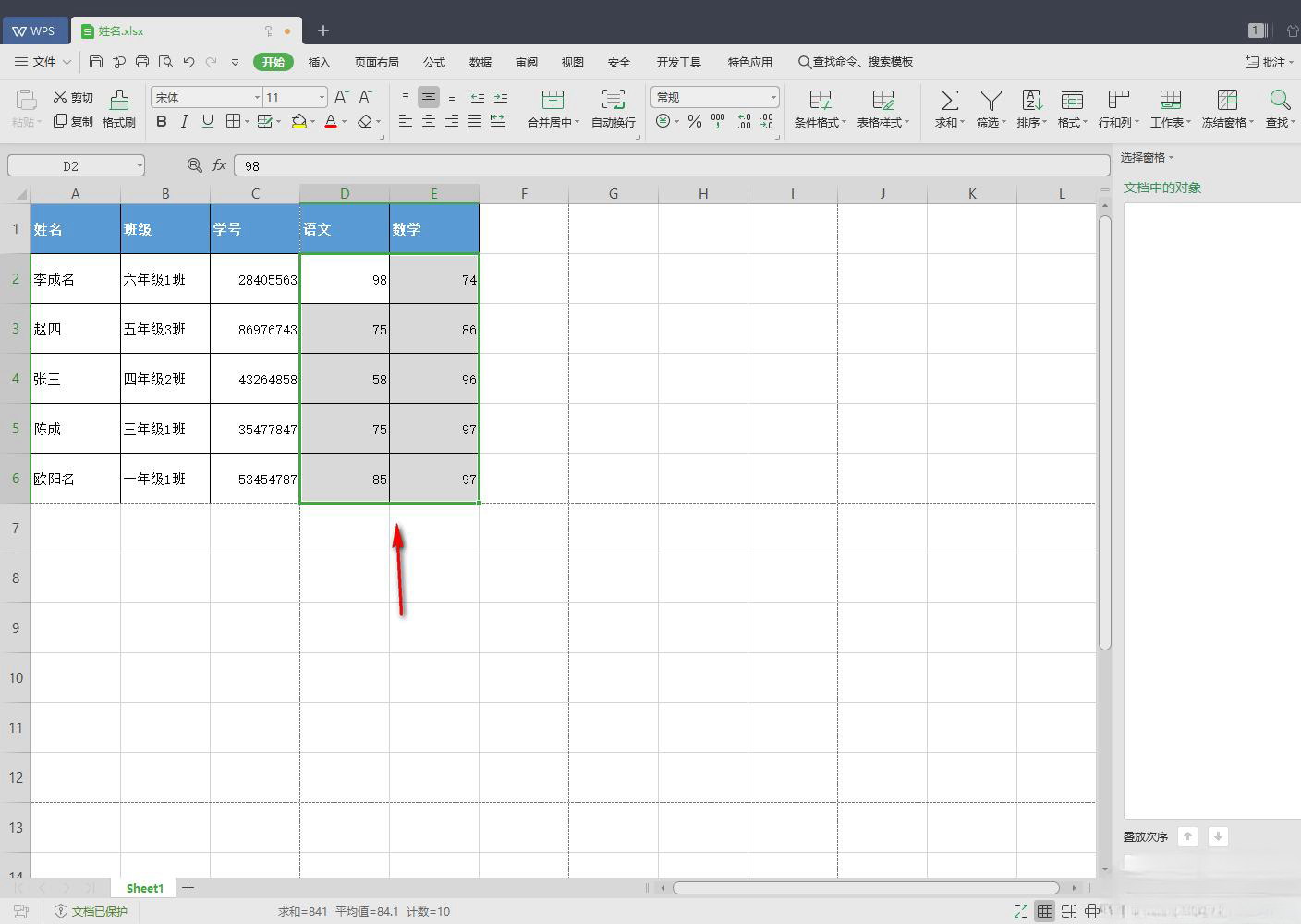
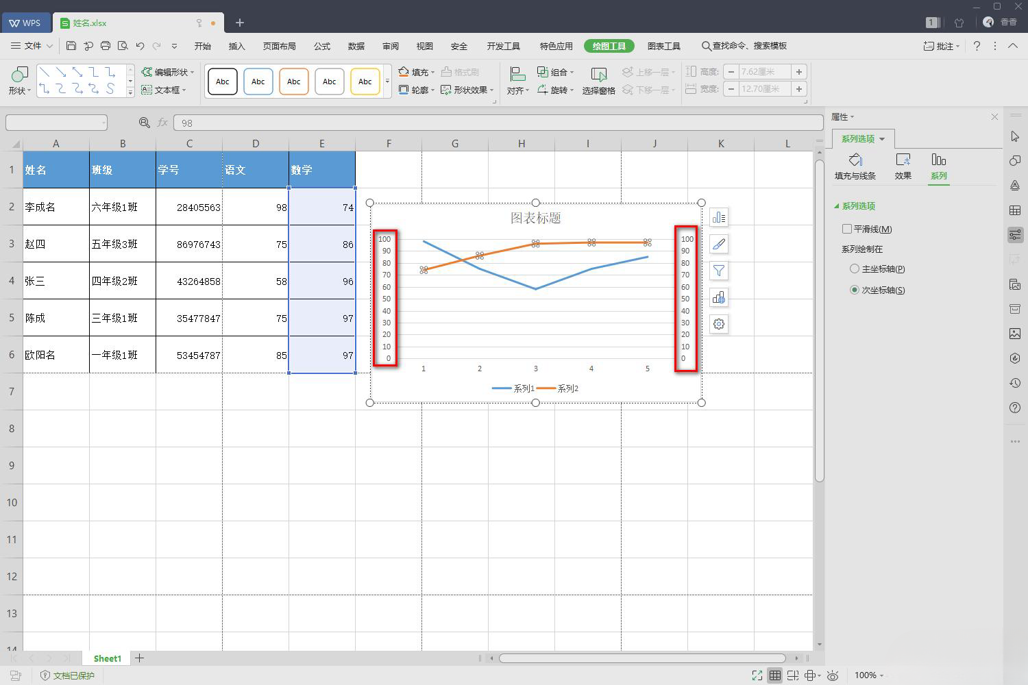
How to set two y-axes in WPS How to set two y-axes in WPS Excel

How to set two y-axes in WPS? When we make statistics on data, we will need to insert charts, pictures, etc., but many users want to set two y-axes when inserting a line chart. So how to do this? Let this site carefully introduce to users the method of setting two Y-axes in WPS Excel. Method for setting two Y-axes in WPS Excel 1. First, we need to open the WPS Excel table content, and then select the data that needs to be statistically analyzed in the line chart.

1. First, move the mouse to the [Insert] option above and click on it.

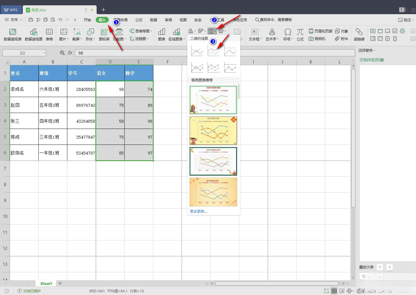
2. At this time, some toolbars will appear below. We select [Line Chart] in the toolbar. After opening the line chart, you can choose a variety of line chart styles. Choose according to your needs.

3. When we insert the line chart into the page, two trend lines will be displayed in the line chart. Then we select one of the trend lines, right-click, and select [ Set data series format].

4. At this time, a properties window will pop up on the right side. In this window, we click and check the [Secondary Axis].

5. Then if you look at the line chart again, you will find that there are Y-axes on both sides of the line chart, then we have set it up successfully.

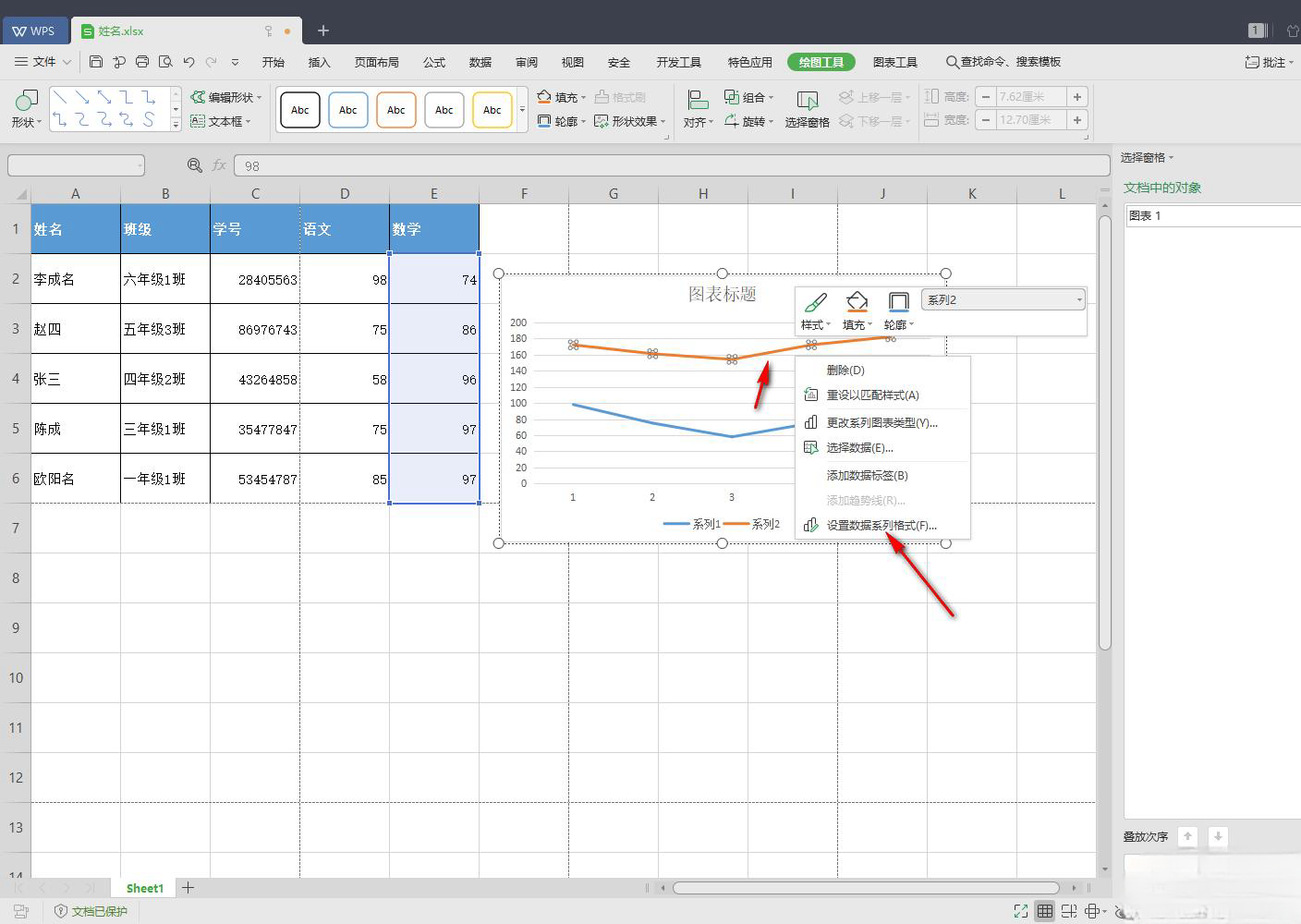
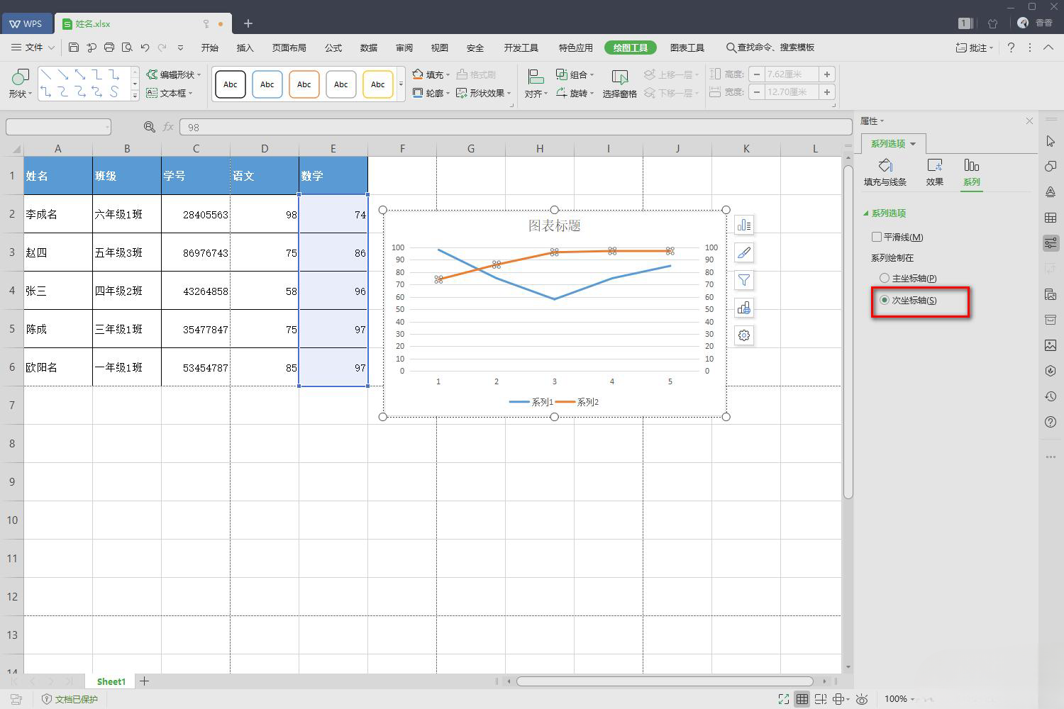
The above is the detailed content of How to set two y-axes in WPS How to set two y-axes in WPS Excel. For more information, please follow other related articles on the PHP Chinese website!