5 Excel Quick Tips You Didn't Know You Needed

Five Excel tips to help you process data efficiently

Many people are familiar with the various features of Excel, but few people understand practical tips that save time and visualize data more effectively. This article will share five tips to help you improve efficiency the next time you use the Microsoft spreadsheet program.

1. Quickly select data area for shortcut keys

Ctrl A shortcut key is well known, but in Excel, it functions differently in different situations.

First, select any cell in the spreadsheet. If the cell is independent of other cells (i.e., there is no data to the left, right, above, or below it, and does not belong to a part of the formatted table), pressing Ctrl A will select the entire spreadsheet.

However, if the selected cell belongs to a data area (such as an unformatted numeric column or a formatted table), pressing Ctrl A will only select that data area. For example, we select cell D6 and press Ctrl A.

This is very useful for formatting only that data range (not the entire worksheet).

Press Ctrl A again and Excel will select the entire spreadsheet.

This is perfect for formatting the entire worksheet at the same time.

This trick improves productivity without using mouse clicks and drags to select data ranges.

2. Add a slicer to quickly filter data

After formatting the data into an Excel table, the Filter button will automatically appear at the top of each column, which you can uncheck or select the Filter button in the Table Design tab to remove or re-add it.

However, a more convenient way to filter is to add slicers, especially when a column is filtered more often than others.

In our example, we expect to filter the "Store" and "Total" columns frequently because they are the main columns in the table, so let's add a slicer for each column.

Select any cell in the table and click "Insert Slicer" in the "Table Design" tab of the ribbon.

Then select the column to which you want to add the slicer and click OK.

Now, you can click and drag to reposition or resize the slicer, or open the Slicer tab to see more options. To go a step further (such as removing the title of the slicer), right-click the relevant slicer and click "Slicer Settings".

Since the slicer automatically displays its data in order (inversely in the original dataset), the data can be analyzed immediately.

When selecting elements in the slicer, pressing the Ctrl key will display all elements at the same time; pressing Alt C will clear all selections in the slicer.

3. Visual trend of creating mini-pictures

You can create highly formatted charts to visualize data graphically, but sometimes you may need a cleaner, smaller space-consuming tool. This is where minimaps come in. Excel offers three types of minimaps .

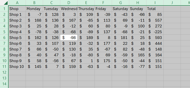
In the following example, we have profit and loss data from different stores for a week and we want to add a visual representation of each store trend in column J.

First, select the cell in column J to display the trend visualization.

Now, in the Insert tab of the ribbon, go to the Minimap group and click Line Chart.

Put the cursor in the "Data Area" field, use the mouse to select the data in the table, and then click OK.

You will immediately see your numbers appear as trendlines.

If the lines are too small and difficult to analyze in full, just increase the size of the cells and columns, and the minimap will automatically fill to the size of the cells.

There are two other types of minimaps that you can use depending on the type of data you want to visualize.

Cylinder minimap presents data in the form of a mini bar chart:

The profit and loss mini chart emphasizes positive and negative values:

After creating a minimap, select any affected cells and use the Minimap tab on the ribbon to make any desired formatting or detail changes. Since they are added together, they will be formatted in the same way at the same time. However, if you want to format them individually, click Ungroup in the Minimap tab. In the following example, we uncombined every other minimap to alternate formatting them.

4. Make full use of preset conditional formats

Another way to visualize and analyze data immediately is to use Excel's preset conditional formatting tool. Setting a conditional formatting rule can take time, and can also cause problems if the rules overlap or conflict with each other, but it is much easier to use the default format.

Select the data in the spreadsheet you want to analyze and click the Conditional Format drop-down menu in the Start tab of the ribbon. There, click "Stripes", "Color Scale", or "Icon Set" and select the style that suits your data.

In our example, we chose the orange stripe, which helps us compare the totals at a glance. Conveniently, since there is a negative number in our data, Excel has automatically formatted the data strips to emphasize the numerical differences.

To clear conditional formatting, select the relevant cell, click Conditional formatting in the Start tab, and then click Clear Rules from Selected Cell.

5. Screenshot data to achieve dynamic update

This is a great way to copy cells on one worksheet to another location (such as a dashboard). Any changes made to the original data will then be reflected in the copied data.

First add the Camera tool to the Quick Access Toolbar (QAT). Click the down arrow to the right of any tab on the ribbon to see if your QAT is enabled. If the Hide Quick Access Toolbar option is available, you have displayed it. Similarly, if you see the "Show Quick Access Toolbar" option, click it to activate your QAT.

Then, click the QAT down arrow and click "More Commands".

Now, select "All Commands" from the "Select Commands from" menu, then scroll to and select "Camera" and click "Add" to add it to your QAT. Then click OK.

You will see the "Camera" icon in QAT.

Select the cell you want to copy in another worksheet or workbook and click the newly added "Camera" icon.

If you want to copy content that is not attached to a cell (such as an image or chart), select the cells behind and around the project. This will copy the selected cell and everything preceding it as an image.

Then, go to the location where you want to copy the data (in the example below, we used worksheet 2), just click once in the appropriate place (in our case, cell A1).

Excel treats it as a picture, so you can use the Picture Format tab on the ribbon to render snapshots accurately.

Before capturing the data as an image, consider removing the grid lines, which will help the image appear tidy in its copy position.

Although this is a picture (usually an unchanged element in the file), if the original data is changed, this will be immediately reflected in the captured version!

---

Learning some of the most useful shortcuts in Excel is another way to improve efficiency, as they avoid switching between using the keyboard and the mouse.

The above is the detailed content of 5 Excel Quick Tips You Didn't Know You Needed. For more information, please follow other related articles on the PHP Chinese website!