

How to Create a Dynamic Table of Contents in Excel

A table of contents is a total game-changer when working with large files – it keeps everything organized and easy to navigate. Unfortunately, unlike Word, Microsoft Excel doesn’t have a simple “Table of Contents” button that adds this handy feature and updates it automatically. No, you’ll have to roll up your sleeves and create a dynamic table of contents yourself. This table will automatically update and contain clickable links, allowing you to add and remove sheets – as well as jump between them – with ease. This guide has all the info you need to create a dynamic table of contents in Excel.
How to Create a Dynamic Table of Contents in Excel
Technically, there are three ways to create a dynamic table of contents (TOC) in Excel. However, only one of them guarantees a fully automated TOC, and that’s Visual Basic for Applications or VBA for short – Microsoft’s native programming language. The other two – traditional formulas and Power Query – will give you a semi-dynamic table of contents in Excel – one that either doesn’t include clickable links or doesn’t update automatically. Since we’re after a fully dynamic Excel table of contents, we’ll use VBA.
If you aren’t particularly VBA-savvy; don’t worry – you just need to follow a few steps. But first – let’s create our table of contents.
Step 1: Click on the “Insert Worksheet” button next to your sheets at the bottom.

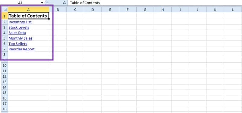
Step 2: Name the sheet “Table of Contents.”

Step 3: Drag the sheet to the first position for better navigation.

Step 4: Enter the names of your sheets in Column A of the “Table of Contents” sheet.

And voilà – you’ve got your table of contents. You can play with the aesthetics of this TOC later – now, we need to make it dynamic. To do so, we’ll need the help of the VBA Editor – a built-in Excel tool that lets you write and run custom codes.
Step 1: Press “Alt + F11” to open the VBA Editor.

Step 2: Go to the “Insert” tab at the top.

Step 3: Select “Module” from the dropdown menu.

Step 4: Copy and paste the following VBA code:
Sub CreateTOC()
Dim ws As Worksheet
Dim toc As Worksheet
Dim i As Integer
‘ Check if TOC sheet already exists, delete if it does
On Error Resume Next
Set toc = ThisWorkbook.Sheets(“Table of Contents”)
On Error GoTo 0
If Not toc Is Nothing Then Application.DisplayAlerts = False: toc.Delete: Application.DisplayAlerts = True
‘ Create new TOC sheet
Set toc = ThisWorkbook.Sheets.Add(Before:=ThisWorkbook.Sheets(1))
toc.Name = “Table of Contents”
‘ Set up TOC header
toc.Cells(1, 1).Value = “Table of Contents”
toc.Cells(1, 1).Font.Bold = True
toc.Cells(1, 1).Font.Size = 14
‘ Loop through all sheets and add hyperlinks
i = 2
For Each ws In ThisWorkbook.Sheets
If ws.Name <> “Table of Contents” Then
toc.Hyperlinks.Add Anchor:=toc.Cells(i, 1), _
Address:=””, _
SubAddress:=”‘” & ws.Name & “‘!A1”, _
TextToDisplay:=ws.Name
i = i + 1
End If
Next ws
‘ Adjust column width
toc.Columns(“A”).AutoFit
End Sub

Step 5: Hit “F5” to run the code.
Step 6: Exit the VBA Editor.
You’ll notice your Excel table of contents is now clickable.
To automatically update your table of contents after changes, you just need to repeat Steps 1 to 6. This will add any new sheets to the list or remove the ones you deleted.

The above is the detailed content of How to Create a Dynamic Table of Contents in Excel. For more information, please follow other related articles on the PHP Chinese website!

Hot AI Tools

Undresser.AI Undress
AI-powered app for creating realistic nude photos

AI Clothes Remover
Online AI tool for removing clothes from photos.

Undress AI Tool
Undress images for free

Clothoff.io
AI clothes remover

AI Hentai Generator
Generate AI Hentai for free.

Hot Article
Hot Tools

Notepad++7.3.1
Easy-to-use and free code editor

SublimeText3 Chinese version
Chinese version, very easy to use

Zend Studio 13.0.1
Powerful PHP integrated development environment

Dreamweaver CS6
Visual web development tools

SublimeText3 Mac version
God-level code editing software (SublimeText3)
Hot Topics
 1382
1382
 52
52

 win11 activation key permanent 2025
Mar 18, 2025 pm 05:57 PM
win11 activation key permanent 2025
Mar 18, 2025 pm 05:57 PM
Article discusses sources for a permanent Windows 11 key valid until 2025, legal issues, and risks of using unofficial keys. Advises caution and legality.
 win11 activation key permanent 2024
Mar 18, 2025 pm 05:56 PM
win11 activation key permanent 2024
Mar 18, 2025 pm 05:56 PM
Article discusses reliable sources for permanent Windows 11 activation keys in 2024, legal implications of third-party keys, and risks of using unofficial keys.
 Acer PD163Q Dual Portable Monitor Review: I Really Wanted to Love This
Mar 18, 2025 am 03:04 AM
Acer PD163Q Dual Portable Monitor Review: I Really Wanted to Love This
Mar 18, 2025 am 03:04 AM
The Acer PD163Q Dual Portable Monitor: A Connectivity Nightmare I had high hopes for the Acer PD163Q. The concept of dual portable displays, conveniently connecting via a single cable, was incredibly appealing. Unfortunately, this alluring idea quic
 ReactOS, the Open-Source Windows, Just Got an Update
Mar 25, 2025 am 03:02 AM
ReactOS, the Open-Source Windows, Just Got an Update
Mar 25, 2025 am 03:02 AM
ReactOS 0.4.15 includes new storage drivers, which should help with overall stability and UDB drive compatibility, as well as new drivers for networking. There are also many updates to fonts support, the desktop shell, Windows APIs, themes, and file
 How to Create a Dynamic Table of Contents in Excel
Mar 24, 2025 am 08:01 AM
How to Create a Dynamic Table of Contents in Excel
Mar 24, 2025 am 08:01 AM
A table of contents is a total game-changer when working with large files – it keeps everything organized and easy to navigate. Unfortunately, unlike Word, Microsoft Excel doesn’t have a simple “Table of Contents” button that adds t
 How to Use Voice Access in Windows 11
Mar 18, 2025 pm 08:01 PM
How to Use Voice Access in Windows 11
Mar 18, 2025 pm 08:01 PM
Detailed explanation of the voice access function of Windows 11: Free your hands and control your computer with voice! Windows 11 provides numerous auxiliary functions to help users with various needs to use the device easily. One of them is the voice access function, which allows you to control your computer completely through voice. From opening applications and files to entering text with voice, everything is at your fingertips, but first you need to set up and learn key commands. This guide will provide details on how to use voice access in Windows 11. Windows 11 Voice Access Function Settings First, let's take a look at how to enable this feature and configure Windows 11 voice access for the best results. Step 1: Open the Settings menu
 Shopping for a New Monitor? 8 Mistakes to Avoid
Mar 18, 2025 am 03:01 AM
Shopping for a New Monitor? 8 Mistakes to Avoid
Mar 18, 2025 am 03:01 AM
Buying a new monitor isn't a frequent occurrence. It's a long-term investment that often moves between computers. However, upgrading is inevitable, and the latest screen technology is tempting. But making the wrong choices can leave you with regret
 New to Multi-Monitors? Don't Make These Mistakes
Mar 25, 2025 am 03:12 AM
New to Multi-Monitors? Don't Make These Mistakes
Mar 25, 2025 am 03:12 AM
Multi-monitor setups boost your productivity and deliver a more immersive experience. However, it's easy for a novice to stumble while assembling the setup and make mistakes. Here are some of the most common ones and how to avoid them.
