

Excel CHOOSEROWS function to extract certain rows from array

In this tutorial, we'll take an in-depth look at the Excel 365 function named CHOOSEROWS and its practical uses.
Suppose you have an Excel worksheet with hundreds of rows from which you want to extract some specific ones, say, all odd or even rows, the first 5 or the last 10 rows, etc. Do you already feel annoyed at the thought of copying and pasting the data manually or writing a VBA code to automate the task? Don't worry! All is much simpler than it seems. Just use the new dynamic array CHOOSEROWS function.
Excel CHOOSEROWS function
The CHOOSEROWS function in Excel is used to extract the specified rows from an array or range.
The syntax is as follows:
CHOOSEROWS(array, row_num1, [row_num2], …)Where:
Array (required) - the source array.
Row_num1 (required) - an integer representing the numeric index of the first row to return.
Row_num2, … (optional) - index numbers of additional rows to return.
Here's how the CHOOSEROWS function works in Excel 365:

CHOOSEROWS function availability
The CHOOSEROWS function is only available in Excel for Microsoft 365 (Windows and Mac) and Excel for the web.
Tip. To get certain columns from a range or array, use the CHOOSECOLS function.
How to use CHOOSEROWS function in Excel
To pull particular rows from a given array, construct a CHOOSEROWS formula in this way:
- For array, you can supply a range of cells or an array of values driven by another formula.
- For row_num, provide a positive or negative integer indicating which row to return. A positive number retrieves a corresponding row from the start of the array, a negative number - from the end of the array. Multiple row numbers can be provided individually in separate arguments or in one argument in the form of an array constant.
As a Excel dynamic array function, CHOOSEROWS handles arrays natively. You enter the formula in the upper-left cell of the destination range, and it automatically spills into as many columns and rows as needed. The result is a single dynamic array, also known as a spill range.
For example, to get rows 2, 4, 6, 8 and 10 from the range A4:D13, the formula is:
=CHOOSEROWS(A4:D13, 2, 4, 6, 8, 10)
Alternatively, you can use an array constant such as {2,4,6,8,10} or {2;4;6;8;10} to specify the desired rows:
=CHOOSEROWS(A4:D13, {2,4,6,8,10})
Or
=CHOOSEROWS(A4:D13, {2;4;6;8;10})

Another way to supply the row numbers is entering them in separate cells, and then using either the individual cell references for several row_num arguments or a range reference for a single row_num argument.
For example:
=CHOOSEROWS(A4:D13, F4, G4, H4)
=CHOOSEROWS(A4:D13, F4:H4)
An advantage of this approach is that it lets you extract any other rows by simply changing the numbers in the predefined cells without editing the formula itself.

Below we will discuss a few more CHOOSEROWS formula examples to handle more specific use cases.
Return rows from the end of an array
To quickly get the last N rows from a range, provide negative numbers for the row_num arguments. This will force the function to count rows from the end of the array.
For instance, to get the last 3 row from the range A4:D13, use this formula:
=CHOOSEROWS(A4:D13, -3, -2, -1)
The result will be a 3-row array where the rows appear in the same ordered as in the referred range.
To return the last 3 rows in the reverse order, from bottom to top, change the order of the row_num arguments like this:
=CHOOSEROWS(A4:D13, -1, -2, -3)

Extract every other row from an array in Excel
To get every other row from a given range, use CHOOSEROWS in combination with a few other functions. The formula will slightly vary depending on whether you are extracting odd or even rows.
To return odd rows such as 1, 3, 5, … the formula takes this form:
=CHOOSEROWS(A4:D13, SEQUENCE(ROUNDUP(ROWS(A4:D13)/2, 0), 1, 1, 2))
To return even rows such as 2, 4, 6, … the formula goes as follows:
=CHOOSEROWS(A4:D13, SEQUENCE(ROUNDDOWN(ROWS(A4:D13)/2, 0), 1, 2, 2))

How this formula works:
In essence, the CHOOSEROWS function returns rows based on an array of sequential odd or even numbers generated by the SEQUENCE function. A detailed formula break-down follows below.
Firstly, you determine how many rows to return. For this, you employ the ROWS function to get the total number of rows in the referenced array, which you divide by 2, and then round the quotient upward or downward to the integer with the help of ROUNDUP or ROUNDDOWN. As this number will later be served to the rows argument of SEQUENCE, rounding is needed to get an integer in case the source range contains an odd number of rows.
As our source range has an even number of rows (10) that is exactly divided by 2, both ROUNDUP(10/2, 0) and ROUNDDOWN(10/2, 0) return the same result, which is 5.
The returned number is served to the SEQUENCE function.
For odd rows:
SEQUENCE(5, 1, 1, 2)
For even rows:
SEQUENCE(5, 1, 2, 2)
The SEQUENCE formula above produces an array of numbers consisting of 5 rows and 1 column, starting at 1 for odd rows (at 2 for even rows), and incremented by 2.
For odd rows, we get this array:
{1;3;5;7;9}
For even rows, we get this one:
{2;4;6;8;10}
The generated array goes to the row_num1 argument of CHOOSEROWS, and you get the desired result:
=CHOOSEROWS(A4:D13, {1;3;5;7;9})
Reverse the order of rows in an array
To flip an array vertically from top to bottom, you can also use the CHOOSEROWS and SEQUENCE functions together. For example:
=CHOOSEROWS(A4:D13, SEQUENCE(ROWS(A4:D13))*-1)
In this formula, we set only the first argument (rows) of SEQUENCE, which equals the total number of rows in the initial array ROWS(A4:D13). The omitted arguments (columns, start, step) default to 1. As a result, SEQUENCE produces an array of sequential numbers such as 1, 2, 3, …, n, where n is the last row in the source array. To make CHOOSEROWS count rows in the down-up direction, the generated sequence is multiplied by -1, so the row_num argument gets an array of negative numbers such as {-1;-2;-3;-4;-5;-6;-7;-8;-9;-10}.
As a result, the order of items in each column is changed from top to bottom:

Extract rows from multiple arrays
To get specific rows from two or more non-contiguous ranges, you first combine them using the VSTACK function, and then pass the merged range to CHOOSEROWS.
For example, to extract the first two rows from the range A4:D8 and the last two rows from the range A12:D16, use this formula:
=CHOOSEROWS(VSTACK(A4:D8, A12:D16), 1, 2, -2, -1)

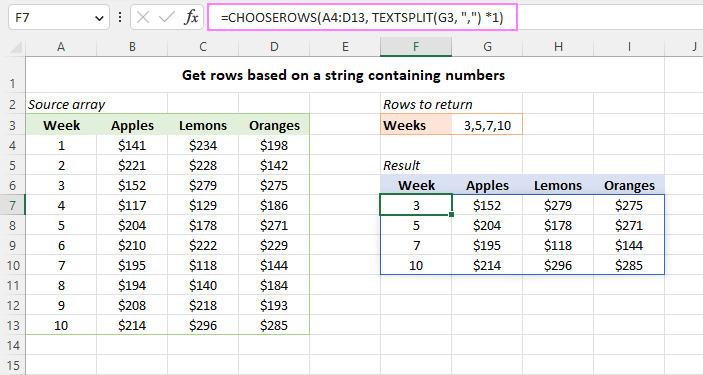
Get rows based on a string containing row numbers
This example shows how to return particular rows by extracting the numbers from an alpha-numeric string.
Suppose you have comma-separated numbers in cell G3 listing the rows of interest. To extract the row numbers from a string, use the TEXTSPLIT function that can split a text string by a given delimiter (comma in our case):
=TEXTSPLIT(G3, ",")
The result is an array of text values such as {"3","5","7","10"}. To convert it to an array of numbers, perform any math operation that does not change the values, say 0 or *1.
=TEXTSPLIT(G3, ",") *1
This produces the numeric array constant {3,5,7,10} that the CHOOSEROWS function needs, so you embed the TEXTSPLIT formula in the 2nd argument:
=CHOOSEROWS(A4:D13, TEXTSPLIT(G3, ",") *1)
As a result, all the specified rows are returned as a single array:
CHOOSEROWS function not working
If the CHOOSEROWS formula results in an error, it's most likely to be one of these reasons.
#VALUE! error
Occurs if the absolute value of any row_num argument is zero or higher than the total number of rows in the array.
#NAME? error
Occurs if the function's name is misspelled or the function is not supported in your Excel. Currently, CHOOSEROWS is only available in Excel 365 and Excel for the web. For more details, read How to fix #NAME error in Excel.
#SPILL! error
Occurs when there are not enough blank cells to fill with the results. To fix it, just clear the obstructing cells. For more information, please see Excel #SPILL! error.
That's how to use the CHOOSEROWS function in Excel to return particular rows from a range or array. Thank you for reading and I hope to see you on our blog next week!
Practice workbook for download
Excel CHOOSEROWS formula - examples (.xlsx file)
The above is the detailed content of Excel CHOOSEROWS function to extract certain rows from array. For more information, please follow other related articles on the PHP Chinese website!

Hot AI Tools

Undresser.AI Undress
AI-powered app for creating realistic nude photos

AI Clothes Remover
Online AI tool for removing clothes from photos.

Undress AI Tool
Undress images for free

Clothoff.io
AI clothes remover

Video Face Swap
Swap faces in any video effortlessly with our completely free AI face swap tool!

Hot Article
Hot Tools

Notepad++7.3.1
Easy-to-use and free code editor

SublimeText3 Chinese version
Chinese version, very easy to use

Zend Studio 13.0.1
Powerful PHP integrated development environment

Dreamweaver CS6
Visual web development tools

SublimeText3 Mac version
God-level code editing software (SublimeText3)
Hot Topics


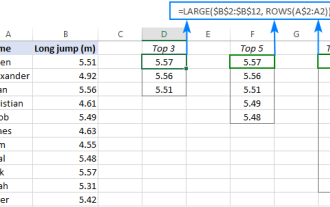 Excel formula to find top 3, 5, 10 values in column or row
Apr 01, 2025 am 05:09 AM
Excel formula to find top 3, 5, 10 values in column or row
Apr 01, 2025 am 05:09 AM
This tutorial demonstrates how to efficiently locate the top N values within a dataset and retrieve associated data using Excel formulas. Whether you need the highest, lowest, or those meeting specific criteria, this guide provides solutions. Findi
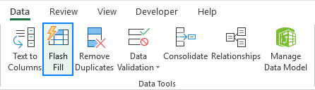 How to use Flash Fill in Excel with examples
Apr 05, 2025 am 09:15 AM
How to use Flash Fill in Excel with examples
Apr 05, 2025 am 09:15 AM
This tutorial provides a comprehensive guide to Excel's Flash Fill feature, a powerful tool for automating data entry tasks. It covers various aspects, from its definition and location to advanced usage and troubleshooting. Understanding Excel's Fla
 How to add calendar to Outlook: shared, Internet calendar, iCal file
Apr 03, 2025 am 09:06 AM
How to add calendar to Outlook: shared, Internet calendar, iCal file
Apr 03, 2025 am 09:06 AM
This article explains how to access and utilize shared calendars within the Outlook desktop application, including importing iCalendar files. Previously, we covered sharing your Outlook calendar. Now, let's explore how to view calendars shared with
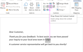 Add a dropdown list to Outlook email template
Apr 01, 2025 am 05:13 AM
Add a dropdown list to Outlook email template
Apr 01, 2025 am 05:13 AM
This tutorial shows you how to add dropdown lists to your Outlook email templates, including multiple selections and database population. While Outlook doesn't directly support dropdowns, this guide provides creative workarounds. Email templates sav
 MEDIAN formula in Excel - practical examples
Apr 11, 2025 pm 12:08 PM
MEDIAN formula in Excel - practical examples
Apr 11, 2025 pm 12:08 PM
This tutorial explains how to calculate the median of numerical data in Excel using the MEDIAN function. The median, a key measure of central tendency, identifies the middle value in a dataset, offering a more robust representation of central tenden
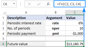 FV function in Excel to calculate future value
Apr 01, 2025 am 04:57 AM
FV function in Excel to calculate future value
Apr 01, 2025 am 04:57 AM
This tutorial explains how to use Excel's FV function to determine the future value of investments, encompassing both regular payments and lump-sum deposits. Effective financial planning hinges on understanding investment growth, and this guide prov
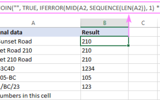 How to remove / split text and numbers in Excel cell
Apr 01, 2025 am 05:07 AM
How to remove / split text and numbers in Excel cell
Apr 01, 2025 am 05:07 AM
This tutorial demonstrates several methods for separating text and numbers within Excel cells, utilizing both built-in functions and custom VBA functions. You'll learn how to extract numbers while removing text, isolate text while discarding numbers
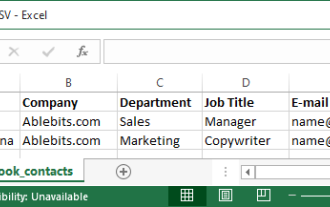 How to import contacts to Outlook (from CSV and PST file)
Apr 02, 2025 am 09:09 AM
How to import contacts to Outlook (from CSV and PST file)
Apr 02, 2025 am 09:09 AM
This tutorial demonstrates two methods for importing contacts into Outlook: using CSV and PST files, and also covers transferring contacts to Outlook Online. Whether you're consolidating data from an external source, migrating from another email pro
