

Excel Data Bars Conditional Formatting with examples

This tutorial shows you how to quickly add and customize colored data bars in Excel to visually compare data. Instead of charts, data bars directly within cells offer a clearer comparison of numerical values. You can choose to display bars alongside the numbers or hide the numbers and show only the bars.
What are Excel Data Bars?
Excel data bars are a built-in conditional formatting feature. They insert colored bars into cells, visually representing the relative size of each cell's value compared to others in the selected range. Longer bars indicate higher values, and shorter bars indicate lower values. This allows for quick identification of highest and lowest values, such as top and bottom performers in sales data. Unlike bar charts, which are separate chart objects, data bars are integrated directly into the cells themselves.

Adding Data Bars in Excel
Follow these steps to add data bars:
- Select the cells you want to format.
- Go to the Home tab, click Conditional Formatting, then select Data Bars.
- Choose either Gradient Fill (for a gradual color change) or Solid Fill (for a single color).
Gradient fill blue data bars will appear immediately:

Solid fill bars allow you to select your preferred color:

To adjust settings, select a formatted cell, go to Conditional Formatting > Manage Rules > Edit Rule, and customize colors and other options. Wider columns improve readability, especially with gradient fills, by separating values from the darker bar sections.
Gradient vs. Solid Fill
- Gradient Fill: Ideal when both bars and values are visible; the lighter bar ends enhance number readability.
- Solid Fill: Best when only bars are displayed, with values hidden.

Creating Custom Data Bars
For personalized data bars, create a custom rule:
- Select the cells.
- Click Conditional Formatting > Data Bars > More Rules.
- In the New Formatting Rule dialog, customize:
- Minimum/Maximum: Choose Automatic (default) or specify values using percentages, numbers, or formulas.
- Fill/Border: Select your preferred colors.
- Bar Direction: Choose from context (default), left-to-right, or right-to-left.
- Show Bar Only: Hide cell values, showing only bars.
Example of custom gradient data bars:

Defining Minimum and Maximum Values
By default, Excel automatically sets minimum and maximum values. For more control:
- Create a new rule (Conditional Formatting > Data Bars > More Rules) or edit an existing one (Conditional Formatting > Manage Rules > Edit).
- In the rule dialog, under Edit the Rule Description, choose your desired Minimum and Maximum options (e.g., percentages).
Example of setting data bar percentages:

Data Bars Based on Formulas
Use formulas to dynamically calculate minimum and maximum values:
-
Minimum:
=MIN($D$3:$D$12)*0.95(sets minimum 5% below the lowest value) -
Maximum:
=MAX($D$3:$D$12)*1.05(sets maximum 5% above the highest value)

Data Bars Based on Another Cell
To apply data bars based on values in different cells, copy the original values to a new column using a formula (e.g., =A1), then apply data bars to the new column and check "Show Bar Only" to hide the numbers.

Data Bars for Negative Values
Data bars work with negative numbers. To use different colors for positive and negative values:
- Select cells, go to Conditional Formatting > Data Bars > More Rules.
- Set positive bar color, then click Negative Value and Axis.
- Customize negative bar colors and axis settings (or choose white for no axis).

Result:

Showing Only Bars (Hiding Values)
To show only bars, check the Show Bar Only box in the Formatting Rule dialog.

This completes the tutorial on adding and customizing data bars in Excel. A practice workbook is available for download.
The above is the detailed content of Excel Data Bars Conditional Formatting with examples. For more information, please follow other related articles on the PHP Chinese website!

Hot AI Tools

Undresser.AI Undress
AI-powered app for creating realistic nude photos

AI Clothes Remover
Online AI tool for removing clothes from photos.

Undress AI Tool
Undress images for free

Clothoff.io
AI clothes remover

AI Hentai Generator
Generate AI Hentai for free.

Hot Article
Hot Tools

Notepad++7.3.1
Easy-to-use and free code editor

SublimeText3 Chinese version
Chinese version, very easy to use

Zend Studio 13.0.1
Powerful PHP integrated development environment

Dreamweaver CS6
Visual web development tools

SublimeText3 Mac version
God-level code editing software (SublimeText3)
Hot Topics
 1384
1384
 52
52

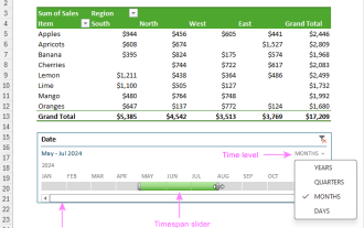 How to create timeline in Excel to filter pivot tables and charts
Mar 22, 2025 am 11:20 AM
How to create timeline in Excel to filter pivot tables and charts
Mar 22, 2025 am 11:20 AM
This article will guide you through the process of creating a timeline for Excel pivot tables and charts and demonstrate how you can use it to interact with your data in a dynamic and engaging way. You've got your data organized in a pivo
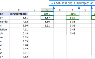 Excel formula to find top 3, 5, 10 values in column or row
Apr 01, 2025 am 05:09 AM
Excel formula to find top 3, 5, 10 values in column or row
Apr 01, 2025 am 05:09 AM
This tutorial demonstrates how to efficiently locate the top N values within a dataset and retrieve associated data using Excel formulas. Whether you need the highest, lowest, or those meeting specific criteria, this guide provides solutions. Findi
 All you need to know to sort any data in Google Sheets
Mar 22, 2025 am 10:47 AM
All you need to know to sort any data in Google Sheets
Mar 22, 2025 am 10:47 AM
Mastering Google Sheets Sorting: A Comprehensive Guide Sorting data in Google Sheets needn't be complex. This guide covers various techniques, from sorting entire sheets to specific ranges, by color, date, and multiple columns. Whether you're a novi
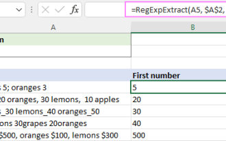 Regex to extract strings in Excel (one or all matches)
Mar 28, 2025 pm 12:19 PM
Regex to extract strings in Excel (one or all matches)
Mar 28, 2025 pm 12:19 PM
In this tutorial, you'll learn how to use regular expressions in Excel to find and extract substrings matching a given pattern. Microsoft Excel provides a number of functions to extract text from cells. Those functions can cope with most
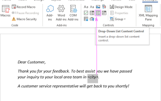 Add a dropdown list to Outlook email template
Apr 01, 2025 am 05:13 AM
Add a dropdown list to Outlook email template
Apr 01, 2025 am 05:13 AM
This tutorial shows you how to add dropdown lists to your Outlook email templates, including multiple selections and database population. While Outlook doesn't directly support dropdowns, this guide provides creative workarounds. Email templates sav
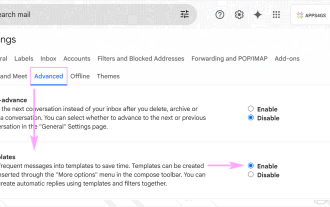 How to enable templates in Gmail — quick setup guide
Mar 21, 2025 pm 12:03 PM
How to enable templates in Gmail — quick setup guide
Mar 21, 2025 pm 12:03 PM
This guide shows you two easy ways to enable email templates in Gmail: using Gmail's built-in settings or installing the Shared Email Templates for Gmail Chrome extension. Gmail templates are a huge time-saver for frequently sent emails, eliminating
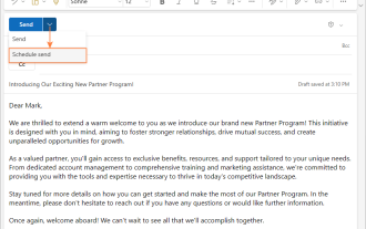 How to schedule send in Outlook
Mar 22, 2025 am 09:57 AM
How to schedule send in Outlook
Mar 22, 2025 am 09:57 AM
Wouldn't it be convenient if you could compose an email now and have it sent at a later, more opportune time? With Outlook's scheduling feature, you can do just that! Imagine that you are working late at night, inspired by a brilliant ide
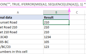 How to remove / split text and numbers in Excel cell
Apr 01, 2025 am 05:07 AM
How to remove / split text and numbers in Excel cell
Apr 01, 2025 am 05:07 AM
This tutorial demonstrates several methods for separating text and numbers within Excel cells, utilizing both built-in functions and custom VBA functions. You'll learn how to extract numbers while removing text, isolate text while discarding numbers
