

Case-sensitive SUMIF and SUMIFS in Excel and Google Sheets

In this tutorial, you will learn how to make a case-sensitive SUMIF or SUMIFS formula in Excel and Google Sheets.
The SUMIF and SUMIFS functions are available in both Microsoft Excel and Google Sheets. And in both applications, they are case-insensitive by nature. To conditionally sum cells treating lowercase and uppercase letters as different characters, you'll have to come up with something else.
Is SUMIF / SUMIFS case sensitive?
No, it is not. In both Excel and Google Sheets, neither SUMIF nor SUMIFS can recognize the letter case. To make sure of this, please consider this simple example:
Supposing you have a list of id's in column A, where uppercase and lowercase letters denote different items. The corresponding sales figures are in column B. The goal is to get a sum of sales for a specific item, say A-01.
With the target id in E1, we construct this classic SUMIF formula:
=SUMIF(A2:A6, E1, B2:B6)
And get an absolutely wrong result :(

Case-sensitive Sum If formula in Excel
To sum cells with one condition considering the letter case, you can use the SUMPRODUCT and EXACT functions together:
SUMPRODUCT(--(EXACT(criteria, range)), sum_range)With the target id in E1(criteria), the items list in A2:A10 (range), and sales numbers in B2:B10 (sum_range), the formulas take these forms:
=SUMPRODUCT(--(EXACT(E1, A2:A10)), B2:B10)
If needed, you can "hardcode" the criteria directly in the formula:
=SUMPRODUCT(--(EXACT("A-01", A2:A10)), B2:B10)

How this formula works:
At the heart of the formula, the EXACT function compares the target item (E1) against each item in the list and returns TRUE if the compared values are exactly the same including the text case, FALSE otherwise:
{TRUE;FALSE;FALSE;FALSE;TRUE;FALSE;TRUE;FALSE;FALSE}
A double unary operator (--) converts TRUE and FALSE into 1 and 0, respectively:
{1;0;0;0;1;0;1;0;0}
The SUMPRODUCT function multiplies the elements of the above array by the corresponding items in B2:B10:
SUMPRODUCT({1;0;0;0;1;0;1;0;0}, {250;155;130;255;160;280;170;285;110})
And because multiplying by 0 gives zero, only the items for which EXACT returned TRUE survive:
SUMPRODUCT({250;0;0;0;160;0;170;0;0})
Finally, SUMPRODUCT adds up the products and outputs the sum.
Case-sensitive Sum Ifs in Excel (with multiple criteria)
In case you are looking for a case-sensitive SUMIFS formula with two or more criteria, you can emulate this behavior by defining an additional range/criteria pair in another EXACT function:
SUMPRODUCT(--(EXACT(criteria1, range1)), --(EXACT(criteria2, range2)), sum_range)For example, to sum sales for a particular item (F1) in a given region (F2), the formula goes as follows:
=SUMPRODUCT(--(EXACT(F1, A2:A10)), --(EXACT(F2, B2:B10)), C2:C10)

Case-sensitive 'Sum If Cell Contains' formula in Excel
In situation when you need to add up values in one column if a cell in another column contains certain text as part of the cell's content, then use the SUMPRODUCT function together with FIND:
SUMPRODUCT(--(ISNUMBER(FIND(criteria, range))), sum_range)For example, to sum sales for the item in E1 (which can match an entire cell in A2:A10 or be just part of the text string), the formula is:
=SUMPRODUCT(--(ISNUMBER(FIND(E1, A2:A10))), B2:B10)

To sum cells based on multiple conditions, add one more ISNUMBER/FIND combo:
SUMPRODUCT(--(ISNUMBER(FIND(criteria1, range1))), --(ISNUMBER(FIND(criteria2, range2))), sum_range)For instance, to get a sum of sales with two conditions (item id in F1 and region in F2), the formula is:
=SUMPRODUCT(--(ISNUMBER(FIND(F1, A2:A10))), --(ISNUMBER(FIND(F2, B2:B10))), C2:C10)
Please note that the formula adds up sales for a specified item in any "north" region, such as North, North-East, or North-West.

How this formula works:
Here, we use the case-sensitive FIND function to search for the target item (E1). When the item is found, the function returns its relative position in the source string, otherwise a #VALUE error.
{2;#VALUE!;#VALUE!;#VALUE!;1;#VALUE!;1;#VALUE!;#VALUE!}
The ISNUMBER function converts any number to TRUE and error values to FALSE:
{TRUE;FALSE;FALSE;FALSE;TRUE;FALSE;TRUE;FALSE;FALSE}
Next, you do "double negation" (--) to coerce the logical values into 1 and 0:
{1;0;0;0;1;0;1;0;0}
Finally, the SUMPRODUCT function multiplies the elements of the two arrays and outputs the result:
SUMPRODUCT({1;0;0;0;1;0;1;0;0}, {250;155;130;255;160;280;170;285;110})
If your formula processes multiple conditions, then SUMPRODUCT will multiply the elements of three or more arrays. In our case, it is:
=SUMPRODUCT({1;0;0;0;1;0;1;0;0}, {1;0;1;1;1;1;0;1;0}, {250;155;130;255;160;280;170;285;110})
SUMIF case-sensitive in Google Sheets
The case-sensitive Sum If formulas that we built for Excel will also work in Google Sheets. Additionally, you can get the Google Sheet's SUMIF function itself to distinguish between uppercase and lowercase characters. Here's how:
SUMIF(ArrayFormula(EXACT(criterion, range)), TRUE, sum_range)Or
SUMIF(ArrayFormula(FIND(criterion, range)), 1, sum_range)For our sample dataset, the real formulas look as follows:
=SUMIF(ArrayFormula(EXACT(E1, A2:A10)), TRUE, B2:B10)
=SUMIF(ArrayFormula(FIND(E1, A2:A10)), 1, B2:B10)

How SUMIF/EXACT formula works:
To make the Google Sheets SUMIF(range, criterion, [sum_range]) function recognize the letter case, we use the following formula for the range argument:
ArrayFormula(EXACT(E1, A2:A10))
ArrayFormula forces EXACT to compare the value in E1 against each value in A2:A10. If an exact match is found, the formula returns TRUE, otherwise – FALSE.
In the range of TRUE and FALSE values, SUMIF searches for TRUE and adds up the corresponding values in B2:B10. That's all!
How SUMIF/FIND formula works:
Here, we use the combination of ArrayFormula and FIND to look for the target value (E1) in the range A2:A10:
ArrayFormula(FIND(E1, A2:A10))
If used separately, the FIND function will stop searching after finding the first match.
Wherever the target value is found, the formula returns 1 (which is its relative position in the search string). For cells where the value is not found, a #VALUE! error is returned.
Next, you use the number 1 as SUMIF's criteria and have the job done :)
SUMIFS case-sensitive in Google Sheets
To sum cells with multiple conditions in Google Sheets, you can use either case-sensitive SUMPRODUCT formulas discussed in Excel's part of our tutorial or Google Sheet's SUMIFS in combination with EXACT or FIND:
SUMIFS(sum_range, ArrayFormula(EXACT(criterion1, range1)), TRUE, ArrayFormula(EXACT(criterion2, range2)), TRUE)Or
SUMIFS(sum_range, ArrayFormula(FIND(criterion1, range1)), 1, ArrayFormula(FIND(criterion2, range2)), 1)As you see, the logic is the same as with the SUMIF function. The difference is that you use two or more range/criterion pairs.
For example, to sum sales for the item in F1 and the region in F2, the formulas are:
=SUMIFS(C2:C10, ArrayFormula(EXACT(F1, A2:A10)), TRUE, ArrayFormula(EXACT(F2, B2:B10)), TRUE)
=SUMIFS(C2:C10, ArrayFormula(FIND(F1, A2:A10)), 1, ArrayFormula(FIND(F2, B2:B10)), 1)

This is how you can create a case-sensitive SUMIF or SUMIFS formula in Excel and Google Sheets. I thank you for reading and hope to see you on our blog next week!
Practice workbooks
Case-sensitive SUMIF / SUMIFS in Excel (.xlsx file) Case-sensitive SUMIF / SUMIFS in Google Sheets (online sheet)
The above is the detailed content of Case-sensitive SUMIF and SUMIFS in Excel and Google Sheets. For more information, please follow other related articles on the PHP Chinese website!

Hot AI Tools

Undresser.AI Undress
AI-powered app for creating realistic nude photos

AI Clothes Remover
Online AI tool for removing clothes from photos.

Undress AI Tool
Undress images for free

Clothoff.io
AI clothes remover

Video Face Swap
Swap faces in any video effortlessly with our completely free AI face swap tool!

Hot Article
Hot Tools

Notepad++7.3.1
Easy-to-use and free code editor

SublimeText3 Chinese version
Chinese version, very easy to use

Zend Studio 13.0.1
Powerful PHP integrated development environment

Dreamweaver CS6
Visual web development tools

SublimeText3 Mac version
God-level code editing software (SublimeText3)
Hot Topics
 1664
1664
 14
1421
52
1315
25
1266
29
1239
24
14
1421
52
1315
25
1266
29
1239
24

 MEDIAN formula in Excel - practical examples
Apr 11, 2025 pm 12:08 PM
MEDIAN formula in Excel - practical examples
Apr 11, 2025 pm 12:08 PM
This tutorial explains how to calculate the median of numerical data in Excel using the MEDIAN function. The median, a key measure of central tendency, identifies the middle value in a dataset, offering a more robust representation of central tenden
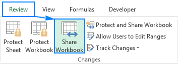 Excel shared workbook: How to share Excel file for multiple users
Apr 11, 2025 am 11:58 AM
Excel shared workbook: How to share Excel file for multiple users
Apr 11, 2025 am 11:58 AM
This tutorial provides a comprehensive guide to sharing Excel workbooks, covering various methods, access control, and conflict resolution. Modern Excel versions (2010, 2013, 2016, and later) simplify collaborative editing, eliminating the need to m
 Google Spreadsheet COUNTIF function with formula examples
Apr 11, 2025 pm 12:03 PM
Google Spreadsheet COUNTIF function with formula examples
Apr 11, 2025 pm 12:03 PM
Master Google Sheets COUNTIF: A Comprehensive Guide This guide explores the versatile COUNTIF function in Google Sheets, demonstrating its applications beyond simple cell counting. We'll cover various scenarios, from exact and partial matches to han
 Excel: If cell contains formula examples
Apr 09, 2025 am 09:04 AM
Excel: If cell contains formula examples
Apr 09, 2025 am 09:04 AM
This tutorial demonstrates various Excel formulas to check if a cell contains specific values, including text, numbers, or parts of strings. It covers scenarios using IF, ISTEXT, ISNUMBER, SEARCH, FIND, COUNTIF, EXACT, SUMPRODUCT, VLOOKUP, and neste
 How to convert Excel to JPG - save .xls or .xlsx as image file
Apr 11, 2025 am 11:31 AM
How to convert Excel to JPG - save .xls or .xlsx as image file
Apr 11, 2025 am 11:31 AM
This tutorial explores various methods for converting .xls files to .jpg images, encompassing both built-in Windows tools and free online converters. Need to create a presentation, share spreadsheet data securely, or design a document? Converting yo
 Google sheets chart tutorial: how to create charts in google sheets
Apr 11, 2025 am 09:06 AM
Google sheets chart tutorial: how to create charts in google sheets
Apr 11, 2025 am 09:06 AM
This tutorial shows you how to create various charts in Google Sheets, choosing the right chart type for different data scenarios. You'll also learn how to create 3D and Gantt charts, and how to edit, copy, and delete charts. Visualizing data is cru
 Excel RANK function and other ways to calculate rank
Apr 09, 2025 am 11:35 AM
Excel RANK function and other ways to calculate rank
Apr 09, 2025 am 11:35 AM
This Excel tutorial details the nuances of the RANK functions and demonstrates how to rank data in Excel based on multiple criteria, group data, calculate percentile rank, and more. Determining the relative position of a number within a list is easi
 How to flip data in Excel columns and rows (vertically and horizontally)
Apr 11, 2025 am 09:05 AM
How to flip data in Excel columns and rows (vertically and horizontally)
Apr 11, 2025 am 09:05 AM
This tutorial demonstrates several efficient methods for vertically and horizontally flipping tables in Excel, preserving original formatting and formulas. While Excel lacks a direct "flip" function, several workarounds exist. Flipping Dat
