ISNA function in Excel with formula examples
Mar 27, 2025 am 11:26 AMThis tutorial explores various methods for using Excel's ISNA function to manage #N/A errors. Excel displays a #N/A error when a lookup value isn't found. The ISNA function helps create more user-friendly formulas and improve worksheet appearance.
- Practical Applications of ISNA
- Combining ISNA with IF
- Using ISNA with VLOOKUP
- Counting #N/A Errors with SUMPRODUCT and ISNA
Excel's ISNA Function
The ISNA function checks for #N/A errors in cells or formulas, returning TRUE if found, and FALSE otherwise. It's compatible with Excel 2000 through 2021 and Excel 365. The syntax is straightforward:
ISNA(value) where value is the cell or formula to check.
A basic ISNA formula using a cell reference:
=ISNA(A2)
This returns TRUE if A2 contains #N/A, and FALSE otherwise.

Practical ISNA Applications
ISNA is most effective when combined with other functions. For example, nest another formula within ISNA's value argument:
ISNA(*your_formula*())
Let's say you're comparing two lists (columns A and D) to find names appearing in both and those unique to list 1. The MATCH function compares A3 with column D:
=MATCH(A3, $D$2:$D$9, 0)
If the name is found, MATCH returns its position; otherwise, #N/A. Wrapping it in ISNA:
=ISNA(MATCH(A3, $D$2:$D$9, 0))
This, when copied down, indicates whether a student (column A) is in column D (TRUE = not found, FALSE = found).

Note: Excel 365 and 2021 users can utilize the more modern XMATCH function.
IF ISNA Formula
Since ISNA only returns TRUE/FALSE, use it with IF for custom messages:
IF(ISNA(…), "*text_if_error*", "*text_if_no_error*")
To show "No failed tests" for students without failed tests (those with #N/A from MATCH):
=IF(ISNA(MATCH(A3,$D$2:$D$9,0)), "No failed tests", "Failed")
This produces clearer results.

ISNA with VLOOKUP
The IF/ISNA combination works with any function returning #N/A. With VLOOKUP:
IF(ISNA(VLOOKUP(…), "*custom_text*", VLOOKUP(…))
This returns custom text if VLOOKUP finds #N/A; otherwise, it returns VLOOKUP's result. To show failed subjects or "No failed tests":
=IF(ISNA(VLOOKUP(A3, $D$3:$E$9, 2, FALSE)), "No failed tests", VLOOKUP(A3, $D$3:$E$9, 2, FALSE))

Excel 2013 offers IFNA for a simpler solution:
=IFNA(VLOOKUP(A3, $D$3:$E$9, 2, FALSE), "-")

Excel 365 and 2021 users can use XLOOKUP:
=XLOOKUP(A3, $D$3:$D$9, $E$3:$E$9, "-")
Counting #N/A Errors with SUMPRODUCT and ISNA
To count #N/A errors in a range:
SUMPRODUCT(--ISNA(*range*))
ISNA creates a TRUE/FALSE array; -- converts to 1s and 0s; SUMPRODUCT sums the result. To count students with no failed tests:
=SUMPRODUCT(--ISNA(MATCH(A3:A14, D2:D9, 0)))

This tutorial demonstrates creating and using ISNA formulas in Excel. Downloadable examples are available.
The above is the detailed content of ISNA function in Excel with formula examples. For more information, please follow other related articles on the PHP Chinese website!

Hot Article

Hot tools Tags

Hot Article

Hot Article Tags

Notepad++7.3.1
Easy-to-use and free code editor

SublimeText3 Chinese version
Chinese version, very easy to use

Zend Studio 13.0.1
Powerful PHP integrated development environment

Dreamweaver CS6
Visual web development tools

SublimeText3 Mac version
God-level code editing software (SublimeText3)
Hot Topics


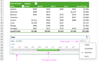 How to create timeline in Excel to filter pivot tables and charts
Mar 22, 2025 am 11:20 AM
How to create timeline in Excel to filter pivot tables and charts
Mar 22, 2025 am 11:20 AM
How to create timeline in Excel to filter pivot tables and charts