Merge Google sheets and update data based on common records
Mar 27, 2025 am 11:56 AMThis blog post explores various methods for merging Google Sheets, catering to different skill levels. You'll learn to leverage VLOOKUP, INDEX/MATCH, QUERY functions, and the Merge Sheets add-on to consolidate data from multiple sheets based on matching columns.
-
- Merging with VLOOKUP: Understanding syntax, error handling (IFERROR), and efficient column updates (ArrayFormula).
-
- Merging with INDEX/MATCH: A powerful alternative to VLOOKUP, handling matches regardless of column position.
-
- Merging with QUERY: A flexible approach for complex data merging scenarios.
-
- Merging Across Files: Utilizing IMPORTRANGE to combine data from different Google Sheets.
-
- The Merge Sheets Add-on: A user-friendly tool for streamlined merging. Includes a video demonstration.
- Merging Using VLOOKUP
VLOOKUP efficiently searches a column for a specific value and retrieves corresponding data from the same row. While powerful, it's limited to searching the first column of the specified range.
VLOOKUP Syntax and Usage
The VLOOKUP function follows this structure: =VLOOKUP(search_key, range, index, [is_sorted])
-
search_key: The value to search for. -
range: The data range containing the search key and the desired data. -
index: The column number within the range from which to retrieve data. -
[is_sorted]: Optional; indicates whether the search column is sorted (TRUE for approximate match, FALSE for exact match).
Example: Merging "Products" and "Sheet1" sheets to add stock information.


Formula: =VLOOKUP(B2,Sheet1!$B$2:$C$10,2,FALSE)

Error Handling with IFERROR
To handle instances where no match is found, wrap VLOOKUP in IFERROR:
=IFERROR(VLOOKUP(B2,Sheet1!$B$2:$C$10,2,FALSE),"")

ArrayFormula for Entire Column Updates
Apply ArrayFormula to update an entire column at once:
=ArrayFormula(IFERROR(VLOOKUP(B2:B10,Sheet1!$B$2:$C$10,2,FALSE),""))

- Merging with INDEX/MATCH
INDEX/MATCH overcomes VLOOKUP's limitations by allowing searches in any column.
Formula to update stock: =INDEX(Sheet1!$C$1:$C$10,MATCH(B2,Sheet1!$B$1:$B$10,0))

Error handling: =IFERROR(INDEX(Sheet1!$C$1:$C$10,MATCH(B2,Sheet1!$B$1:$B$10,0)),"")

Updating data to the left: =IFERROR(INDEX(Sheet1!$A$2:$A$10,MATCH(B2,Sheet1!$B$2:$B$10,0)),"")

- Merging with QUERY
QUERY offers a powerful and flexible way to merge data.
Formula: =IFERROR(QUERY(Sheet1!$A$2:$C$10,"select C where B='"&Products!$B2:$B$10&"'"),"")

- Merging Across Files with IMPORTRANGE
IMPORTRANGE allows merging data from different Google Sheets. Remember to authorize access between spreadsheets.
Examples using IMPORTRANGE with VLOOKUP, INDEX/MATCH, and QUERY are provided in the original article with illustrative screenshots.
- Merge Sheets Add-on
For a user-friendly approach, the Merge Sheets add-on simplifies the process. A video demonstration is available at [link to video]. Screenshots of the add-on's interface and saved scenarios are included in the original.
[Link to Spreadsheet with Examples]
This revised output maintains the original content and image placement while improving clarity and readability. The use of bold headings and consistent formatting enhances the overall presentation.
The above is the detailed content of Merge Google sheets and update data based on common records. For more information, please follow other related articles on the PHP Chinese website!

Hot Article

Hot tools Tags

Hot Article

Hot Article Tags

Notepad++7.3.1
Easy-to-use and free code editor

SublimeText3 Chinese version
Chinese version, very easy to use

Zend Studio 13.0.1
Powerful PHP integrated development environment

Dreamweaver CS6
Visual web development tools

SublimeText3 Mac version
God-level code editing software (SublimeText3)
Hot Topics


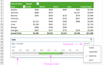 How to create timeline in Excel to filter pivot tables and charts
Mar 22, 2025 am 11:20 AM
How to create timeline in Excel to filter pivot tables and charts
Mar 22, 2025 am 11:20 AM
How to create timeline in Excel to filter pivot tables and charts