

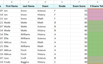
How to highlight top 3, 5, 10 values in Excel

This tutorial demonstrates how to highlight top or bottom N values in an Excel dataset using conditional formatting. We'll explore Excel's built-in tools and create custom rules using formulas for greater flexibility.
Methods for Highlighting Top/Bottom Values:
We'll cover three approaches: using built-in rules, enhancing formatting options, and employing formulas for dynamic control.
1. Built-in Top/Bottom Rules:
This is the quickest method for highlighting a fixed number (e.g., top 3, bottom 10) of values.
- Select your data range.
- Go to the Home tab, click Conditional Formatting, then Top/Bottom Rules, and choose either Top 10 Items or Bottom 10 Items.
- Specify the number of items to highlight and select a formatting style. You can customize the formatting using Custom Format.

2. Enhanced Formatting Options:
For more control over the appearance, create a new rule:
- Select your data range.
- Go to Conditional Formatting > New Rule.
- Choose "Format only top or bottom ranked values".
- Select Top or Bottom, enter the number of values, and click Format to customize the font, border, and fill.

3. Formula-Based Conditional Formatting:
This provides the most flexibility, allowing you to change the number of highlighted values without modifying the rule itself.
- Create input cells (e.g., F2 for top N, F3 for bottom N). Enter the desired number of values.
- Select your data range (e.g., A2:C8).
- Go to Conditional Formatting > New Rule > "Use a formula to determine which cells to format".
- Use the following formulas:
-
Top N:
=A2>=LARGE($A$2:$C$8,$F$2) -
Bottom N:
=A2
-
Top N:
- Click Format to choose your formatting style.

These formulas use LARGE and SMALL functions to dynamically determine the threshold values. Absolute references ($) lock the range and input cells, while the relative reference (A2) allows the formula to apply correctly to each cell in the range.
Highlighting Rows Based on Column Values:
To highlight entire rows based on top/bottom N values in a specific column (e.g., column B):
-
Top N Rows:
=$B2>=LARGE($B$2:$B$15,$E$2) -
Bottom N Rows:
=$B2
Apply these formulas to the entire table (excluding the header row).

Highlighting Top N Values in Each Row:
For highlighting the top N values within each row across multiple columns, use this formula:
=B2>=LARGE($B2:$G2,3)
Apply this to the entire numeric data range (e.g., B2:G10).

This formula uses relative row references and absolute column references to correctly compare values within each row.
Downloadable Practice Workbook: Highlight top or bottom values in Excel (.xlsx file)
The above is the detailed content of How to highlight top 3, 5, 10 values in Excel. For more information, please follow other related articles on the PHP Chinese website!

Hot AI Tools

Undresser.AI Undress
AI-powered app for creating realistic nude photos

AI Clothes Remover
Online AI tool for removing clothes from photos.

Undress AI Tool
Undress images for free

Clothoff.io
AI clothes remover

AI Hentai Generator
Generate AI Hentai for free.

Hot Article
Hot Tools

Notepad++7.3.1
Easy-to-use and free code editor

SublimeText3 Chinese version
Chinese version, very easy to use

Zend Studio 13.0.1
Powerful PHP integrated development environment

Dreamweaver CS6
Visual web development tools

SublimeText3 Mac version
God-level code editing software (SublimeText3)
Hot Topics
 1376
1376
 52
52

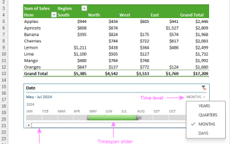 How to create timeline in Excel to filter pivot tables and charts
Mar 22, 2025 am 11:20 AM
How to create timeline in Excel to filter pivot tables and charts
Mar 22, 2025 am 11:20 AM
This article will guide you through the process of creating a timeline for Excel pivot tables and charts and demonstrate how you can use it to interact with your data in a dynamic and engaging way. You've got your data organized in a pivo
 how to sum a column in excel
Mar 14, 2025 pm 02:42 PM
how to sum a column in excel
Mar 14, 2025 pm 02:42 PM
The article discusses methods to sum columns in Excel using the SUM function, AutoSum feature, and how to sum specific cells.
 how to do a drop down in excel
Mar 12, 2025 am 11:53 AM
how to do a drop down in excel
Mar 12, 2025 am 11:53 AM
This article explains how to create drop-down lists in Excel using data validation, including single and dependent lists. It details the process, offers solutions for common scenarios, and discusses limitations such as data entry restrictions and pe
 how to make pie chart in excel
Mar 14, 2025 pm 03:32 PM
how to make pie chart in excel
Mar 14, 2025 pm 03:32 PM
The article details steps to create and customize pie charts in Excel, focusing on data preparation, chart insertion, and personalization options for enhanced visual analysis.
 how to make a table in excel
Mar 14, 2025 pm 02:53 PM
how to make a table in excel
Mar 14, 2025 pm 02:53 PM
Article discusses creating, formatting, and customizing tables in Excel, and using functions like SUM, AVERAGE, and PivotTables for data analysis.
 how to calculate mean in excel
Mar 14, 2025 pm 03:33 PM
how to calculate mean in excel
Mar 14, 2025 pm 03:33 PM
Article discusses calculating mean in Excel using AVERAGE function. Main issue is how to efficiently use this function for different data sets.(158 characters)
 how to add drop down in excel
Mar 14, 2025 pm 02:51 PM
how to add drop down in excel
Mar 14, 2025 pm 02:51 PM
Article discusses creating, editing, and removing drop-down lists in Excel using data validation. Main issue: how to manage drop-down lists effectively.
 All you need to know to sort any data in Google Sheets
Mar 22, 2025 am 10:47 AM
All you need to know to sort any data in Google Sheets
Mar 22, 2025 am 10:47 AM
Mastering Google Sheets Sorting: A Comprehensive Guide Sorting data in Google Sheets needn't be complex. This guide covers various techniques, from sorting entire sheets to specific ranges, by color, date, and multiple columns. Whether you're a novi
