

Excel NPER function with formula examples

In this tutorial, you will learn: What does nper mean in Excel? How to use the NPER function to calculate the number of periods required to pay off a loan or the number of investments needed to earn the target amount? And more!
When building corporate funds, financial analysts often wish to know how long it will take to reach the desired corpus. When applying for a loan, you may want to find out how many payments are required to repay it in full. For such tasks, Excel provides the NPER function, which stands for "number of periods".
Excel NPER function
NPER is an Excel financial function that calculates the number of payment periods for a loan or investment based on equal periodic payments and a constant interest rate.
The function is available in all versions Excel 365, Excel 2019, Excel 2016, Excel 2013, Excel 2010 and Excel 2007.
The syntax is as follows:
NPER(rate, pmt, pv, [fv], [type])Where:
- Rate (required) - the interest rate per period. If you pay once a year, specify an annual interest rate; if you pay each month, provide a monthly interest rate, etc.
- Pmt (required) - the amount paid each period. Normally, it includes principal and interest, but no taxes or fees.
- Pv (required) - the present value of the loan or investment, i.e. how much a series of future cash flows is worth right now.
- Fv (optional) - the future value of the loan or investment after the last payment. If omitted, defaults to 0.
-
Type (optional) - specifies when the payments are due:
- 0 or omitted (default) - at the end of an accounting period
- 1 - at the beginning of an accounting period
4 things you should know about NPER function
To effectively use the Excel NPER function in your worksheets and avoid common mistakes, please remember the following things:
- Use positive numbers for inflows (any amounts you receive) and negative numbers for outflows (any amounts that you pay).
- If the present value (pv) is zero or omitted, the future value (fv) must be included.
- The rate argument can be entered as percentage or decimal number, e.g. 5% or 0.05.
- Be sure to supply rate corresponding to periods. For instance, if a loan is to be paid monthly at an annual interest rate of 8%, then use 8%/12 or 0.08/12 for the rate argument.
Basic NPER formula in Excel
Knowing the theory, let's build an NPER formula in its simplest form to get the number of periods to clear the loan based on the following data:
- Annual interest rate (rate): C2
- Yearly payment (pmt): C3
- Loan amount (pv): C4
Putting the arguments together, we get this simple formula:
=NPER(C2, C3, C4)
The optional [fv] and [type] arguments are omitted because the future value is irrelevant in this case, and the payments are due at the end of the year, which is the default type.
Assuming the $10,000 loan is given to you at an 8% annual interest rate, and you will pay $3,800 to the bank each year, the formula shows that you will have to make 3 yearly payments to pay back the loan amount.
Please notice that pmt is a negative number because it is outgoing cash.

If you enter a periodic payment as a positive number, then put the minus sign before the pmt argument directly in the formula:
=NPER(C2, -C3, C4)

How to use NPER function in Excel - formula examples
Below, you will find a few more examples of Excel NPER formula that show how to calculate the number of payment periods for different scenarios.
Calculate the number of periodic payments for a loan
Most mortgage and other long-term loans are paid in monthly installments. Some other are paid quarterly or semiannually. The question is - how do you find the number of periodic payments required to pay back the total loan amount?
The key is to convert an annual interest rate to a periodic rate. For this, simply divide the yearly rate by the number of periods per year:
Monthly payments: rate = annual interest rate / 12
Quarterly payments: rate = annual interest rate / 4
Semiannual payments: rate = annual interest rate / 2
Let's assume you borrowed $10,000 at an 8% annual interest rate, with a monthly payment of $500.
We start with entering the data in the corresponding cells:
- Annual interest rate (C2): 8%
- Monthly payment (C3): -500
- Loan amount (C4): 10,000
To get a correct value for the rate argument, divide C2 by 12. And you'll come up with the following formula to calculate the number of monthly payments on the loan:
=NPER(C2/12, C3, C4)
The result shows that it will take 22 months (or 1 year and 10 months) to pay off the loan:

If you make quarterly payments, use C2/4 for rate to force NPER to return periods in quarters:
=NPER(C2/4, C3, C4)

Alternatively, you can enter the number of periods per year in a separate cell (C5) and divide the annual interest rate (C2) by that cell:
=NPER(C2/C5, C3, C4)

Calculate NPER based on present and future values
When investing or saving money, you generally know how much you'd like to earn at the end of the term. In this case, you can include the desired future value (fv) in the formula.
Suppose you wish to invest $1,000 at an annual interest rate of 3% and make an additional contribution of $500 at the end of each month. Your goal is to reach $10,000.
To find the number of monthly investments, input the following data in predefined cells:
- Annual interest rate (C2): 3%
- Monthly payment (C3): -500
- Present value (C4): -1,000
- Future value (C5): 10,000
- Periods per year (C6): 12
Enter this formula in C8:
=NPER(C2/C6, C3, C4, C5)
And you will see that it takes 18 monthly investments to reach the target amount:

Please notice that:
- For rate, we divide an annual interest rate by the number of periods per year (months in our case) to get the NPER function to return periods in months.
- Both pmt and pv are negative numbers because they represent an outflow.
- It is assumed that payments are due at the end of the period, so the type argument is omitted.
A universal formula to find NPER in Excel
Handling specific cases was easy, wasn't it? How about building a general formula that does a perfect job of calculating NPER in Excel whether you are borrowing or saving and no matter how often you make payments? For this, we will be using the NPER function in its full form and allocate cells for all the arguments, including the optional ones. In our case, that will be:
- Annual interest rate (rate) - C2
- Periodic payment (pmt) - C3
- Present value (pv) - C4
- Future value (fv) - C5
- When payments are due (type) - C6
- Periods per year - C7
Let's say you wish to invest initial $10,000 at an annual interest rate of 5%, and then make an additional payment of $1,000 at the beginning of each quarter, aiming to reach $50,000. How many quarterly payments you will have to make?
To get the correct periodic rate, we divide the annual interest rate (C2) by the number of periods per year (C7). For the other arguments, simply supply the corresponding cell references:
=NPER(C2/C7, C3, C4, C5, C6)

Tips:
- To leave less room for errors, you can create a drop-down list that only allows 0 and 1 values for the type argument.
- Normally, when you borrow money, you make the payment at the end of a period to let interest accumulate (type is set to 0). When trying to save, you are interested to get the money in as soon as possible so you will accumulate the interest, which is why you pay at the beginning of a period (type is set to 1).
How to get NPER function to return a whole number
In the above examples, the calculated number of periods is displayed as an integer because the formula cell is formatted to show no decimal places. If you format the cell to show one or more decimal places, you will see that the result of NPER is actually a decimal number:

In real life, however, there can be no decimal periods. In such situations, the last payment will just be lower than in previous periods.
To get the correct number of required periods, you can wrap your NPER formula in the ROUNDUP function that rounds the value upward to a specified number of digits. Since we want the result to be an integer, we set the num_digits argument to zero:
ROUNDUP(NPER(), 0)With the annual interest rate in C2, payment amount in C3 and loan amount in C4, the formula takes this form:
=ROUNDUP(NPER(C2, C3, C4), 0)
As you see, the full number of periods is 4, and not 3 as you may think looking at the above screenshot. You will just have to pay a very small amount in the 4th year.

Excel NPER function not working
If your NPER formula returns an error or a wrong result, most likely that will be one of the following.
#NUM! error
Occurs if the specified future value (fv) can never be achieved with a given interest rate (rate) and payment (pmt). To get a valid result, try to increase a periodic interest rate and/or a payment amount.
#VALUE! error
Occurs if any argument is non-numeric. To fix the error, make sure that no numbers used in a formula are formatted as text. For more information, please see How to convert text to number.
The result of NPER function is a negative number
Usually, this problem occurs when outgoing payments are represented by positive numbers. For example, when calculating payment periods for a loan, supply the loan amount (pv) as a positive number and the periodic payment (pmt) as a negative number. When investing or saving money, the initial investment (pv) and periodic payment (pmt) should both be negative and the future value (fv) positive.
That's how to how to find NPER in Excel. I thank you for reading and hope to see you on our blog next week!
Practice workbook for download
Examples of NPER formula in Excel (.xlsx file)
The above is the detailed content of Excel NPER function with formula examples. For more information, please follow other related articles on the PHP Chinese website!

Hot AI Tools

Undresser.AI Undress
AI-powered app for creating realistic nude photos

AI Clothes Remover
Online AI tool for removing clothes from photos.

Undress AI Tool
Undress images for free

Clothoff.io
AI clothes remover

Video Face Swap
Swap faces in any video effortlessly with our completely free AI face swap tool!

Hot Article
Hot Tools

Notepad++7.3.1
Easy-to-use and free code editor

SublimeText3 Chinese version
Chinese version, very easy to use

Zend Studio 13.0.1
Powerful PHP integrated development environment

Dreamweaver CS6
Visual web development tools

SublimeText3 Mac version
God-level code editing software (SublimeText3)
Hot Topics
 1664
1664
 14
1421
52
1315
25
1266
29
1239
24
14
1421
52
1315
25
1266
29
1239
24

 MEDIAN formula in Excel - practical examples
Apr 11, 2025 pm 12:08 PM
MEDIAN formula in Excel - practical examples
Apr 11, 2025 pm 12:08 PM
This tutorial explains how to calculate the median of numerical data in Excel using the MEDIAN function. The median, a key measure of central tendency, identifies the middle value in a dataset, offering a more robust representation of central tenden
 Excel shared workbook: How to share Excel file for multiple users
Apr 11, 2025 am 11:58 AM
Excel shared workbook: How to share Excel file for multiple users
Apr 11, 2025 am 11:58 AM
This tutorial provides a comprehensive guide to sharing Excel workbooks, covering various methods, access control, and conflict resolution. Modern Excel versions (2010, 2013, 2016, and later) simplify collaborative editing, eliminating the need to m
 Google Spreadsheet COUNTIF function with formula examples
Apr 11, 2025 pm 12:03 PM
Google Spreadsheet COUNTIF function with formula examples
Apr 11, 2025 pm 12:03 PM
Master Google Sheets COUNTIF: A Comprehensive Guide This guide explores the versatile COUNTIF function in Google Sheets, demonstrating its applications beyond simple cell counting. We'll cover various scenarios, from exact and partial matches to han
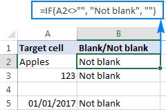 Excel: If cell contains formula examples
Apr 09, 2025 am 09:04 AM
Excel: If cell contains formula examples
Apr 09, 2025 am 09:04 AM
This tutorial demonstrates various Excel formulas to check if a cell contains specific values, including text, numbers, or parts of strings. It covers scenarios using IF, ISTEXT, ISNUMBER, SEARCH, FIND, COUNTIF, EXACT, SUMPRODUCT, VLOOKUP, and neste
 How to convert Excel to JPG - save .xls or .xlsx as image file
Apr 11, 2025 am 11:31 AM
How to convert Excel to JPG - save .xls or .xlsx as image file
Apr 11, 2025 am 11:31 AM
This tutorial explores various methods for converting .xls files to .jpg images, encompassing both built-in Windows tools and free online converters. Need to create a presentation, share spreadsheet data securely, or design a document? Converting yo
 Google sheets chart tutorial: how to create charts in google sheets
Apr 11, 2025 am 09:06 AM
Google sheets chart tutorial: how to create charts in google sheets
Apr 11, 2025 am 09:06 AM
This tutorial shows you how to create various charts in Google Sheets, choosing the right chart type for different data scenarios. You'll also learn how to create 3D and Gantt charts, and how to edit, copy, and delete charts. Visualizing data is cru
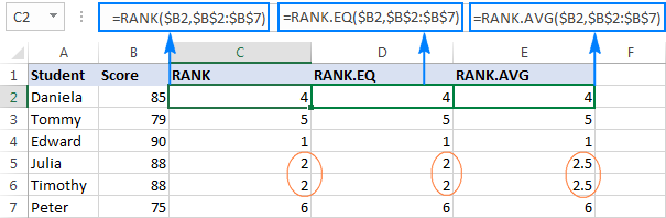 Excel RANK function and other ways to calculate rank
Apr 09, 2025 am 11:35 AM
Excel RANK function and other ways to calculate rank
Apr 09, 2025 am 11:35 AM
This Excel tutorial details the nuances of the RANK functions and demonstrates how to rank data in Excel based on multiple criteria, group data, calculate percentile rank, and more. Determining the relative position of a number within a list is easi
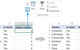 How to flip data in Excel columns and rows (vertically and horizontally)
Apr 11, 2025 am 09:05 AM
How to flip data in Excel columns and rows (vertically and horizontally)
Apr 11, 2025 am 09:05 AM
This tutorial demonstrates several efficient methods for vertically and horizontally flipping tables in Excel, preserving original formatting and formulas. While Excel lacks a direct "flip" function, several workarounds exist. Flipping Dat
