Excel UNIQUE function - fastest way to find unique values
The tutorial looks at how to get unique values in Excel by using the UNIQUE function and dynamic arrays. You will learn a simple formula to find unique values in a column or row, in multiple columns, based on conditions, and a lot more.
In the previous versions of Excel, extracting a list of unique values was a hard challenge. We have a special article that shows how to find uniques that occur just once, extract all distinct items in a list, ignore blanks, and more. Each task required a combined use of several functions and a multi-line array formula that only Excel gurus can fully understand.
The introduction of the UNIQUE function in Excel 365 has changed everything! What used to be a rocket science becomes as easy as ABC. Now, you don't need to be a formula expert to get unique values from a range, based on one or multiple criteria, and arrange the results in alphabetical order. All is done with simple formulas that everyone can read and adjust for your own needs.
Excel UNIQUE function
The UNIQUE function in Excel returns a list of unique values from a range or array. It works with any data type: text, numbers, dates, times, etc.
The function is categorized under Dynamic Arrays functions. The result is a dynamic array that automatically spills into the neighboring cells vertically or horizontally.
The syntax of the Excel UNIQUE function is as follows:
UNIQUE(array, [by_col], [exactly_once])Where:
Array (required) - the range or array from which to return unique values.
By_col (optional) - a logical value indicating how to compare data:
- TRUE - compares data across columns.
- FALSE or omitted (default) - compares data across rows.
Exactly_once (optional) - a logical value that defines what values are considered unique:
- TRUE - returns values that occur only once, which is the database notion of unique.
- FALSE or omitted (default) - returns all distinct (different) values in the range or array.
Note. Currently the UNIQUE function is only available in Excel for Microsoft 365 and Excel 2021. Excel 2019, 2016 and earlier do not support dynamic array formulas, so the UNIQUE function is not available in these versions.
Basic UNIQUE formula in Excel
Below is an Excel unique values formula in its simplest form.
The goal is to extract a list of unique names from the range B2:B10. For this, we enter the following formula in D2:
=UNIQUE(B2:B10)
Please notice that the 2nd and 3rd arguments are omitted because the defaults work perfectly in our case - we are comparing the rows against each other and wish to return all the different names in the range.
When you press the Enter key to complete the formula, Excel will output the first found name in D2 spilling the other names into the cells below. As the result, you have all the unique values in a column:

In case your data is across the columns from B2 to I2, set the 2nd argument to TRUE to compare the columns against each other:
=UNIQUE(B2:I2,TRUE)
Type the above formula in B4, press Enter, and the results will spill horizontally into the cells to the right. Thus, you'll get the unique values in a row:

Tip. To find unique values in a multi-column arrays and return them in one column or row, use UNIQUE together with the TOCOL or TOROW function as shown in the below examples:
- Extract unique values from a multi-column range into a column
- Pull unique values from a multi-column range into a row
Excel UNIQUE function - tips and notes
UNIQUE is a new function and like other dynamic array functions has a few specificities that you should be aware of:
- If the array returned by UNIQUE is the final result (i.e. not passed to another function), Excel dynamically creates an appropriately sized range and populates it with the results. The formula needs to be entered only in one cell. It is important that you have enough empty cells down and/or to the right of the cell where you enter the formula, otherwise a #SPILL error occurs.
- The results update automatically when the source data changes. However, new entries that are added outside of the referenced array are not included in the formula unless you change the array reference. If you want the array to respond to the resizing of the source range automatically, then convert the range to an Excel table and use structured references, or create a dynamic named range.
- Dynamic arrays between different Excel files only work when both workbooks are open. If the source workbook is closed, a linked UNIQUE formula will return a #REF! error.
- Like other dynamic array functions, UNIQUE can only be used within a normal range, not a table. When put within Excel tables, it returns a #SPILL! error.
How to find unique values in Excel - formula examples
The below examples show some practical uses of the UNIQUE function in Excel. The main idea is to extract unique values or remove duplicates, depending on your viewpoint, in the simplest possible way.
Extract unique values that occur only once
To get a list of values that appear in the specified range exactly once, set the 3rd argument of UNIQUE to TRUE.
For example, to pull the names that are on the winners list one time, use this formula:
=UNIQUE(B2:B10,,TRUE)
Where B2:B10 is the source range and the 2nd argument (by_col) is FALSE or omitted because our data is organized in rows.

Find distinct values that occur more than once
If you are pursuing an opposite goal, i.e. are looking to get a list of values that appear in a given range more than one time, then use the UNIQUE function together with FILTER and COUNTIF:
UNIQUE(FILTER(range, COUNTIF(range, range)>1))For example, to extract different names that occur in B2:B10 more than once, you can use this formula:
=UNIQUE(FILTER(B2:B10, COUNTIF(B2:B10, B2:B10)>1))

How this formula works:
At the heart of the formula, the FILTER function filters out duplicate entries based on the count of occurrences, returned by the COUNTIF function. In our case, the result of COUNTIF is this array of counts:
{4;1;3;4;4;1;3;4;3}
The comparison operation (>1) changes the above array to TRUE and FALSE values, where TRUE represents the items that appear more than once:
{TRUE;FALSE;TRUE;TRUE;TRUE;FALSE;TRUE;TRUE;TRUE}
This array is handed off to FILTER as the include argument, telling the function which values to include in the resulting array:
{"Andrew";"David";"Andrew";"Andrew";"David";"Andrew";"David"}
As you can notice, only the values corresponding to TRUE survive.
The above array goes to the array argument of UNIQUE, and after removing duplicates it outputs the final result:
{"Andrew";"David"}
Tip. In a similar fashion, you can filter unique values that occur more than twice (>2), more than three times (>3), etc. For this, simply change the number in the logical comparison.
Find unique values in multiple columns (unique rows)
In situation when you want to compare two or more columns and return the unique values between them, include all the target columns in the array argument.
For instance, to return the unique First name (column A) and Last name (column B) of the winners, we enter this formula in E2:
=UNIQUE(A2:B10)
Pressing the Enter key yields the following results:

To get unique rows, i.e. the entries with the unique combination of values in columns A, B and C, this is the formula to use:
=UNIQUE(A2:C10)
Amazingly simple, isn't it? :)

Get a list of unique values sorted in alphabetical order
How do you usually alphabetize in Excel? Right, by using the inbuilt Sort or Filter feature. The problem is you need to re-sort every time your source data changes, because unlike Excel formulas that recalculate automatically with every change in the worksheet, the features have to be re-applied manually.
With the introduction of dynamic array functions this problem is gone! What you need to do is simply warp the SORT function around a regular UNIQUE formula, like this:
SORT(UNIQUE(array))For example, to extract unique values in columns A through C and arrange the results from A to Z, use this formula:
=SORT(UNIQUE(A2:C10))
Compared to the above example, the output is a lot easier to perceive and work with. For instance, we can clearly see that Andrew and David have been winners in two different sports.

Tip. In this example, we sorted the values in the 1st column from A to Z. These are the defaults of the SORT function, therefore the optional sort_index and sort_order arguments are omitted. If you want to sort the results by some other column or in a different order (from Z to A or from highest to smallest) set the 2nd and 3rd arguments as explained in the SORT function tutorial.
Find unique values in multiple columns and concatenate into one cell
When searching in multiple columns, by default, the Excel UNIQUE function outputs each value in a separate cell. Perhaps, you'll find it more convenient to have the results in a single cell?
To achieve this, instead of referencing the entire range, use the ampersand (&) to concatenate the columns and put the desired delimiter in between.
As an example, we are concatenating the first names in A2:A10 and the last names in B2:B10, separating the values with a space character (" "):
=UNIQUE(A2:A10&" "&B2:B10)
As the result, we have a list of full names in one column:

Get a list of unique values based on criteria
To extract unique values with condition, use the Excel UNIQUE and FILTER functions together:
- The FILTER function limits the data only to values that meet the condition.
- The UNIQUE function removes duplicates from the filtered list.
Here's the generic version of the filtered unique values formula:
UNIQUE(FILTER(array, criteria_range = criteria))For this example, let's get a list of winners in a specific sport. For starters, we input the sport of interest in some cell, say F1. And then, use the below formula to get the unique names:
=UNIQUE(FILTER(A2:B10, C2:C10=F1))
Where A2:B10 is a range to search for unique values and C2:C10 is the range to check for the criteria.

Filter unique values based on multiple criteria
To filter unique values with two or more conditions, use the expressions like shown below to construct the required criteria for the FILTER function:
UNIQUE(FILTER(array, (criteria_range1 = criteria1) * (criteria_range2 = criteria2)))The result of the formula is a list of unique entries for which all of the specified conditions are TRUE. In terms of Excel, this is called the AND logic.
To see the formula in action, let's get a list of unique winners for the sport in G1 (criteria 1) and under the age in G2 (criteria 2).
With the source range in A2:B10, sports in C2:C10 (criteria_range 1) and ages in D2:D10 (criteria_range 2), the formula takes this form:
=UNIQUE(FILTER(A2:B10, (C2:C10=G1) * (D2:D10<g2></g2>
And returns exactly the results we are looking for:

How this formula works:
Here's a high-level explanation of the formula's logic:
In the include argument of the FILTER function, you supply two or more range/criteria pairs. The result of each logical expression is an array of TRUE and FALSE values. The multiplication of the arrays coerces the logical values to numbers and produces an array of 1's and 0's. Since multiplying by zero always gives zero, only the entries that meet all the conditions have 1 in the final array. The FILTER function filters out the items corresponding to 0 and hands off the results to UNIQUE.
For more information, please see FILTER with multiple criteria using AND logic.
Filter unique values with multiple OR criteria
To get a list of unique values based on multiple OR criteria, i.e. when this OR that criterion is TRUE, add the logical expressions instead of multiplying them:
UNIQUE(FILTER(array, (criteria_range1 = criteria1) (criteria_range2 = criteria2)))For example, to show the winners in either Soccer or Hockey, you can use this formula:
=UNIQUE(FILTER(A2:B10, (C2:C10="Soccer") (C2:C10="Hockey")))
If needed, you can of course enter the criteria in separate cells and refer to those cells like shown below:
=UNIQUE(FILTER(A2:B10, (C2:C10=G1) (C2:C10=G2)))

How this formula works:
Just like when testing multiple AND criteria, you place several logical expressions in the include argument of the FILTER function, each of which returns an array of TRUE and FALSE values. When these arrays are added up, the items for which one or more criteria is TRUE will have 1, and the items for which all the criteria are FALSE will have 0. As the result, any entry that meets any single condition makes it into the array that is handed over to UNIQUE.
For more information, please see FILTER with multiple criteria using OR logic.
Get unique values in Excel ignoring blanks
If you are working with a data set that contains some gaps, a list of uniques obtained with a regular formula is likely to have an empty cell and/or zero value. This happens because the Excel UNIQUE function is designed to return all distinct values in a range, including blanks. So, if your source range has both zeros and blank cells, the unique list will contain 2 zeros, one representing a blank cell and the other - a zero value itself. Additionally, if the source data contains empty strings returned by some formula, the uique list will also include an empty string ("") that visually looks like a blank cell:

To get a list of unique values without blanks, this is what you need to do:
- Filter out blank cells and empty strings by using the FILTER function.
- Utilize the UNIQUE function to limit results to unique values only.
In a generic form, the formula looks as follows:
UNIQUE(FILTER(range, range""))In this example, the formula in D2 is:
=UNIQUE(FILTER(B2:B12, B2:B12""))
As the result, Excel returns a list of unique names without empty cells:

Note. In case the original data contains zeros, one zero value will be included in the unique list.
Find unique values in specific columns
Sometimes you may want to extract unique values from two or more columns that are not adjacent to each other. At times, you may also want to re-order the columns in the resulting list. Both tasks can be fulfilled with help of CHOOSE function.
UNIQUE(CHOOSE({1,2,…}, range1, range2))From our sample table, suppose you wish to get a list of winners based on the values in columns A and C and arrange the results in this order: first a sport (column C), and then a sportsman name (column A). To have it done, we construct this formula:
=UNIQUE(CHOOSE({1,2}, C2:C10, A2:A10))
And get the following result:

How this formula works:
The CHOOSE function returns a 2-dimentional array of values from the specified columns. In our case, it also swaps the order of columns.
{"Basketball","Andrew"; "Basketball","Betty"; "Volleyball","David"; "Basketball","Andrew"; "Hockey","Andrew"; "Soccer","Robert"; "Volleyball","David"; "Hockey","Andrew"; "Basketball","David"}
From the above array, the UNIQUE function returns a list of unique records.
Find unique values and handle errors
The UNIQUE formulas we've discussed in this tutorial work just perfect… provided there is at least one value that meets the specified criteria. If the formula does not find anything, a #CALC! error occurs:

To prevent this from happening, simply wrap your formula in the IFERROR function.
For example, if no unique values meeting the criteria are found, you can display nothing, i.e. an empty string (""):
=IFERROR(UNIQUE(FILTER(A2:B10, (C2:C10=G1) * (D2:D10<g2></g2>
Or you can clearly inform your users that no results are found:
=IFERROR(UNIQUE(FILTER(A2:B10, (C2:C10=G1) * (D2:D10<g2 results>
<p><img  src="/static/imghw/default1.png" data-src="https://img.php.cn/upload/article/000/000/000/174347193269059.png" class="lazy" alt="Excel UNIQUE function - fastest way to find unique values" ></p>


<h2 id="Excel-UNIQUE-function-not-working">Excel UNIQUE function not working</h2>
<p>As you have seen, the emergence of the UNIQUE function has made finding unique values in Excel incredibly easy. If all of a sudden your formula results in an error, it's most likely to be one of the following.</p>

<h3 id="NAME-error">#NAME? error</h3>
<p>Occurs if you use a UNIQUE formula in an Excel version where this function is not supported.</p>
<p>Currently, the UNIQUE function is only available in Excel 365 and 2021. If you have a different version, you may find an appropriate solution in this tutorial: How to get unique values in Excel 2019, Excel 2016 and earlier.</p>
<p>The #NAME? error in supported versions indicates that the function's name is misspelled. For more details, see How to fix #NAME error in Excel.


</p>
<h3 id="SPILL-error">#SPILL error</h3>
<p>Occurs if one or more cells in the spill range are not completely blank.
</p>
<p><img  src="/static/imghw/default1.png" data-src="https://img.php.cn/upload/article/000/000/000/174347193419432.png" class="lazy" alt="Excel UNIQUE function - fastest way to find unique values" ></p></g2>
To fix the error, just clear or delete non-empty cells. To see exactly which cells are getting in the way, click the error indicator, and then click Select Obstructing Cells. For more information, please see #SPILL! error in Excel - causes and fixes.
That's how to find unique values in Excel. I thank you for reading and hope to see you on our blog next week!
Practice workbook for download
Excel unique values formula examples (.xlsx file)
The above is the detailed content of Excel UNIQUE function - fastest way to find unique values. For more information, please follow other related articles on the PHP Chinese website!

Hot AI Tools

Undresser.AI Undress
AI-powered app for creating realistic nude photos

AI Clothes Remover
Online AI tool for removing clothes from photos.

Undress AI Tool
Undress images for free

Clothoff.io
AI clothes remover

AI Hentai Generator
Generate AI Hentai for free.

Hot Article

Hot Tools

Notepad++7.3.1
Easy-to-use and free code editor

SublimeText3 Chinese version
Chinese version, very easy to use

Zend Studio 13.0.1
Powerful PHP integrated development environment

Dreamweaver CS6
Visual web development tools

SublimeText3 Mac version
God-level code editing software (SublimeText3)

Hot Topics
 1382
1382
 52
52
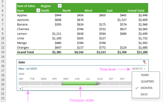 How to create timeline in Excel to filter pivot tables and charts
Mar 22, 2025 am 11:20 AM
This article will guide you through the process of creating a timeline for Excel pivot tables and charts and demonstrate how you can use it to interact with your data in a dynamic and engaging way. You've got your data organized in a pivo
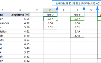 Excel formula to find top 3, 5, 10 values in column or row
Apr 01, 2025 am 05:09 AM
This tutorial demonstrates how to efficiently locate the top N values within a dataset and retrieve associated data using Excel formulas. Whether you need the highest, lowest, or those meeting specific criteria, this guide provides solutions. Findi
 All you need to know to sort any data in Google Sheets
Mar 22, 2025 am 10:47 AM
Mastering Google Sheets Sorting: A Comprehensive Guide Sorting data in Google Sheets needn't be complex. This guide covers various techniques, from sorting entire sheets to specific ranges, by color, date, and multiple columns. Whether you're a novi
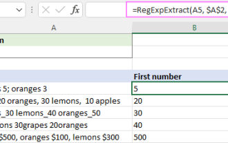 Regex to extract strings in Excel (one or all matches)
Mar 28, 2025 pm 12:19 PM
In this tutorial, you'll learn how to use regular expressions in Excel to find and extract substrings matching a given pattern. Microsoft Excel provides a number of functions to extract text from cells. Those functions can cope with most
 Add a dropdown list to Outlook email template
Apr 01, 2025 am 05:13 AM
This tutorial shows you how to add dropdown lists to your Outlook email templates, including multiple selections and database population. While Outlook doesn't directly support dropdowns, this guide provides creative workarounds. Email templates sav
 How to enable templates in Gmail — quick setup guide
Mar 21, 2025 pm 12:03 PM
This guide shows you two easy ways to enable email templates in Gmail: using Gmail's built-in settings or installing the Shared Email Templates for Gmail Chrome extension. Gmail templates are a huge time-saver for frequently sent emails, eliminating
 How to schedule send in Outlook
Mar 22, 2025 am 09:57 AM
Wouldn't it be convenient if you could compose an email now and have it sent at a later, more opportune time? With Outlook's scheduling feature, you can do just that! Imagine that you are working late at night, inspired by a brilliant ide
 How to remove / split text and numbers in Excel cell
Apr 01, 2025 am 05:07 AM
This tutorial demonstrates several methods for separating text and numbers within Excel cells, utilizing both built-in functions and custom VBA functions. You'll learn how to extract numbers while removing text, isolate text while discarding numbers


