

How to count unique values in Excel: with criteria, ignoring blanks

The tutorial looks at how to leverage the new dynamic array functions to count unique values in Excel: formula to count unique entries in a column, with multiple criteria, ignoring blanks, and more.
A couple of years ago, we discussed various ways to count unique and distinct values in Excel. But like any other software program, Microsoft Excel continuously evolves, and new features appear with almost every release. Today, we will look at how counting unique values in Excel can be done with the recently introduced dynamic array functions. If you have not used any of these functions yet, you will be amazed to see how much simpler the formulas become in terms of building and convenience to use.
Note. All the formulas discussed in this tutorial rely on the UNIQUE function, which is only available in Excel 365 and Excel 2021. If you are using Excel 2019, Excel 2016 or earlier, please check out this article for solutions.
Count unique values in column
The easiest way to count unique values in a column is to use the UNIQUE function together with the COUNTA function:
COUNTA(UNIQUE(range))The formula works with this simple logic: UNIQUE returns an array of unique entries, and COUNTA counts all the elements of the array.
As an example, let's count unique names in the range B2:B10:
=COUNTA(UNIQUE(B2:B10))
The formula tells us that there are 5 different names in the winners list:

Tip. In this example, we count unique text values, but you can use this formula for other data types too including numbers, dates, times, etc.
Count unique values that occur just once
In the previous example, we counted all the different (distinct) entries in a column. This time, we want to know the number of unique records that occur only once. To have it done, build your formula in this way:
To get a list of one-time occurrences, set the 3rd argument of UNIQUE to TRUE:
UNIQUE(B2:B10,,TRUE))
To count the unique one-time occurrences, nest UNIQUE in the ROW function:
ROWS(UNIQUE(B2:B10,,TRUE))
Please note that COUNTA won't work in this case because it counts all non-blank cells, including error values. So, if no results are found, UNIQUE would return an error, and COUNTA would count it as 1, which is wrong!
To handle possible errors, wrap the IFERROR function around your formula and instruct it to output 0 if any error occurs:
=IFERROR(ROWS(UNIQUE(B2:B10,,TRUE)), 0)
As the result, you get a count based on the database concept of unique:

Count unique rows in Excel
Now that you know how to count unique cells in a column, any idea on how to find the number of unique rows?
Here's the solution:
ROWS(UNIQUE(range))The trick is to "feed" the entire range to UNIQUE so that it finds the unique combinations of values in multiple columns. After that, you simply enclose the formula in the ROWS function to calculate the number of rows.
For example, to count the unique rows in the range A2:C10, we use this formula:
=ROWS(UNIQUE(A2:C10))

Count unique entries ignoring blank cells
To count unique values in Excel ignoring blanks, employ the FILTER function to filter out empty cells, and then warp it in the already familiar COUNTA UNIQUE formula:
COUNTA(UNIQUE(FILTER(range, range"")))With the source data in B2:B11, the formula takes this form:
=COUNTA(UNIQUE(FILTER(B2:B11, B2:B11"")))
The screenshot below shows the result:

Count unique values with criteria
To extract unique values based on certain criteria, you again use the UNIQUE and FILTER functions together as explained in this example. And then, you use the ROWS function to count unique entries and IFERROR to trap all kinds of errors and replace them with 0:
IFERROR(ROWS(UNIQUE(range, criteria_range=criteria))), 0)For example, to find how many different winners there are in a specific sport, use this formula:
=IFERROR(ROWS(UNIQUE(FILTER(A2:A10,B2:B10=E1))), 0)
Where A2:A10 is a range to search for unique names (range), B2:B10 are the sports in which the winners compete (criteria_range), and E1 is the sport of interest (criteria).

Count unique values with multiple criteria
The formula for counting unique values based on multiple criteria is pretty much similar to the above example, though the criteria are constructed a bit differently:
IFERROR(ROWS(UNIQUE(range, (criteria_range1=criteria1) * (criteria_range2=criteria2)))), 0)Those who are curious to know the inner mechanics, can find the explanation of the formula's logic here: Find unique values based on multiple criteria.
In this example, we are going to find out how many different winners there are in a specific sport in F1 (criteria 1) and under the age in F2 (criteria 2). For this, we are using this formula:
=IFERROR(ROWS(UNIQUE(FILTER(A2:A10, (B2:B10=F1) * (C2:C10<f2></f2>
Where A2:B10 is the list of names (range), C2:C10 are sports (criteria_range 1) and D2:D10 are ages (criteria_range 2).

That's how to count unique values in Excel with the new dynamic array functions. I am sure you appreciate how much simpler all the solutions become. Anyway, thank you for reading and hope to see you on our blog next week!
Practice workbook for download
Count unique values formula examples (.xlsx file)
The above is the detailed content of How to count unique values in Excel: with criteria, ignoring blanks. For more information, please follow other related articles on the PHP Chinese website!

Hot AI Tools

Undresser.AI Undress
AI-powered app for creating realistic nude photos

AI Clothes Remover
Online AI tool for removing clothes from photos.

Undress AI Tool
Undress images for free

Clothoff.io
AI clothes remover

AI Hentai Generator
Generate AI Hentai for free.

Hot Article
Hot Tools

Notepad++7.3.1
Easy-to-use and free code editor

SublimeText3 Chinese version
Chinese version, very easy to use

Zend Studio 13.0.1
Powerful PHP integrated development environment

Dreamweaver CS6
Visual web development tools

SublimeText3 Mac version
God-level code editing software (SublimeText3)
Hot Topics
 1382
1382
 52
52

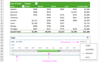 How to create timeline in Excel to filter pivot tables and charts
Mar 22, 2025 am 11:20 AM
How to create timeline in Excel to filter pivot tables and charts
Mar 22, 2025 am 11:20 AM
This article will guide you through the process of creating a timeline for Excel pivot tables and charts and demonstrate how you can use it to interact with your data in a dynamic and engaging way. You've got your data organized in a pivo
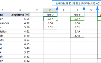 Excel formula to find top 3, 5, 10 values in column or row
Apr 01, 2025 am 05:09 AM
Excel formula to find top 3, 5, 10 values in column or row
Apr 01, 2025 am 05:09 AM
This tutorial demonstrates how to efficiently locate the top N values within a dataset and retrieve associated data using Excel formulas. Whether you need the highest, lowest, or those meeting specific criteria, this guide provides solutions. Findi
 All you need to know to sort any data in Google Sheets
Mar 22, 2025 am 10:47 AM
All you need to know to sort any data in Google Sheets
Mar 22, 2025 am 10:47 AM
Mastering Google Sheets Sorting: A Comprehensive Guide Sorting data in Google Sheets needn't be complex. This guide covers various techniques, from sorting entire sheets to specific ranges, by color, date, and multiple columns. Whether you're a novi
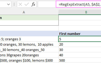 Regex to extract strings in Excel (one or all matches)
Mar 28, 2025 pm 12:19 PM
Regex to extract strings in Excel (one or all matches)
Mar 28, 2025 pm 12:19 PM
In this tutorial, you'll learn how to use regular expressions in Excel to find and extract substrings matching a given pattern. Microsoft Excel provides a number of functions to extract text from cells. Those functions can cope with most
 Add a dropdown list to Outlook email template
Apr 01, 2025 am 05:13 AM
Add a dropdown list to Outlook email template
Apr 01, 2025 am 05:13 AM
This tutorial shows you how to add dropdown lists to your Outlook email templates, including multiple selections and database population. While Outlook doesn't directly support dropdowns, this guide provides creative workarounds. Email templates sav
 How to enable templates in Gmail — quick setup guide
Mar 21, 2025 pm 12:03 PM
How to enable templates in Gmail — quick setup guide
Mar 21, 2025 pm 12:03 PM
This guide shows you two easy ways to enable email templates in Gmail: using Gmail's built-in settings or installing the Shared Email Templates for Gmail Chrome extension. Gmail templates are a huge time-saver for frequently sent emails, eliminating
 How to schedule send in Outlook
Mar 22, 2025 am 09:57 AM
How to schedule send in Outlook
Mar 22, 2025 am 09:57 AM
Wouldn't it be convenient if you could compose an email now and have it sent at a later, more opportune time? With Outlook's scheduling feature, you can do just that! Imagine that you are working late at night, inspired by a brilliant ide
 How to remove / split text and numbers in Excel cell
Apr 01, 2025 am 05:07 AM
How to remove / split text and numbers in Excel cell
Apr 01, 2025 am 05:07 AM
This tutorial demonstrates several methods for separating text and numbers within Excel cells, utilizing both built-in functions and custom VBA functions. You'll learn how to extract numbers while removing text, isolate text while discarding numbers
