

How to subtract in Excel: cells, columns, percentages, dates and times

The tutorial shows how to do subtraction in Excel by using the minus sign and SUM function. You will also learn how to subtract cells, entire columns, matrices and lists.
Subtraction is one of the four basic arithmetic operations, and every primary school pupil knows that to subtract one number from another you use the minus sign. This good old method works in Excel too. What kind of things can you subtract in your worksheets? Just any things: numbers, percentages, days, months, hours, minutes and seconds. You can even subtract matrices, text strings and lists. Now, let's take a look at how you can do all this.
Subtraction formula in Excel (minus formula)
For the sake of clarity, the SUBTRACT function in Excel does not exist. To perform a simple subtraction operation, you use the minus sign (-).
The basic Excel subtraction formula is as simple as this:
=number1-number2For example, to subtract 10 from 100, write the below equation and get 90 as the result:
=100-10
To enter the formula in your worksheet, do the following:
- In a cell where you want the result to appear, type the equality sign (=).
- Type the first number followed by the minus sign followed by the second number.
- Complete the formula by pressing the Enter key.
Like in math, you can perform more than one arithmetic operation within a single formula.
For example, to subtract a few numbers from 100, type all those numbers separated by a minus sign:
=100-10-20-30
To indicate which part of the formula should be calculated first, use parentheses. For example:
=(100-10)/(80-20)
The screenshot below shows a few more formulas to subtract numbers in Excel:

How to subtract cells in Excel
To subtract one cell from another, you also use the minus formula but supply cell references instead of actual numbers:
=cell_1 - cell_2For example, to subtract the number in B2 from the number in A2, use this formula:
=A2-B2
You do not necessarily have to type cell references manually, you can quickly add them to the formula by selecting the corresponding cells. Here's how:
- In the cell where you want to output the difference, type the equals sign (=) to begin your formula.
- Click on the cell containing a minuend (a number from which another number is to be subtracted). Its reference will be added to the formula automatically (A2).
- Type a minus sign (-).
- Click on the cell containing a subtrahend (a number to be subtracted) to add its reference to the formula (B2).
- Press the Enter key to complete your formula.
And you will have a result similar to this:

How to subtract multiple cells from one cell in Excel
To subtract multiple cells from the same cell, you can use any of the following methods.
Method 1. Minus sign
Simply type several cell references separated by a minus sign like we did when subtracting multiple numbers.
For example, to subtract cells B2:B6 from B1, construct a formula in this way:
=B1-B2-B3-B4-B5-B6

Method 2. SUM function
To make your formula more compact, add up the subtrahends (B2:B6) using the SUM function, and then subtract the sum from the minuend (B1):
=B1-SUM(B2:B6)

Method 3. Sum negative numbers
As you may remember from a math course, subtracting a negative number is the same as adding it. So, make all the numbers you want to subtract negative (for this, simply type a minus sign before a number), and then use the SUM function to add up the negative numbers:
=SUM(B1:B6)

How to subtract columns in Excel
To subtract 2 columns row-by-row, write a minus formula for the topmost cell, and then drag the fill handle or double-click the plus sign to copy the formula to the entire column.
As an example, let's subtract numbers in column C from the numbers in column B, beginning with row 2:
=B2-C2

Due to the use of relative cell references, the formula will adjust properly for each row:

Subtract the same number from a column of numbers
To subtract one number from a range of cells, enter that number in some cell (F1 in this example), and subtract cell F1 from the first cell in the range:
=B2-$F$1
The key point is to lock the reference for the cell to be subtracted with the $ sign. This creates an absolute cell reference that does not change no matter where the formula is copied. The first reference (B2) is not locked, so it changes for each row.
As the result, in cell C3 you will have the formula =B3-$F$1; in cell C4 the formula will change to =B4-$F$1, and so on:

If the design of your worksheet does not allow for an extra cell to accommodate the number to be subtracted, nothing prevents you from hardcoding it directly in the formula:
=B2-150
How to subtract percentage in Excel
If you want to simply subtract one percentage from another, the already familiar minus formula will work a treat. For example:
=100%-30%
Or, you can enter the percentages in individual cells and subtract those cells:
=A2-B2

If you wish to subtract percentage from a number, i.e. decrease number by percentage, then use this formula:
=Number * (1 - %)For example, here's how you can reduce the number in A2 by 30%:
=A2*(1-30%)
Or you can enter the percentage in an individual cell (say, B2) and refer to that cell by using an absolute reference:
=A2*(1-$B$2)

For more information, please see How to calculate percentage in Excel.
How to subtract dates in Excel
The easiest way to subtract dates in Excel is to enter them in individual cells, and subtract one cell from the other:
=End_date - Start_date
You can also supply dates directly in your formula with the help of the DATE or DATEVALUE function. For example:
=DATE(2018,2,1)-DATE(2018,1,1)
=DATEVALUE("2/1/2018")-DATEVALUE("1/1/2018")
More information about subtracting dates can be found here:
- How to add and subtract dates in Excel
- How to calculate days between dates in Excel
How to subtract time in Excel
The formula for subtracting time in Excel is built in a similar way:
=End_time-Start_timeFor example, to get the difference between the times in A2 and B2, use this formula:
=A2-B2
For the result to display correctly, be sure to apply the Time format to the formula cell:

You can achieve the same result by supplying the time values directly in the formula. For Excel to understand the times correctly, use the TIMEVALUE function:
=TIMEVALUE("4:30 PM")-TIMEVALUE("12:00 PM")
For more information about subtracting times, please see:
- How to calculate time in Excel
- How to add & subtract time to show over 24 hours, 60 minutes, 60 seconds
How to do matrix subtraction in Excel
Suppose you have two sets of values (matrices) and you want to subtract the corresponding elements of the sets like shown in the screenshot below:
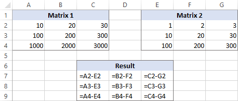
Here's how you can do this with a single formula:
- Select a range of empty cells that has the same number of rows and columns as your matrices.
- In the selected range or in the formula bar, type the matrix subtraction formula:
=(A2:C4)-(E2:G4) - Press Ctrl Shift Enter to make it an array formula.


The results of the subtraction will appear in the selected range. If you click on any cell in the resulting array and look at the formula bar, you will see that the formula is surrounded by {curly braces}, which is a visual indication of array formulas in Excel:

If you do not like using array formulas in your worksheets, then you can insert a normal subtraction formula in the top leftmost cell and copy in rightwards and downwards to as many cells as your matrices have rows and columns.
In this example, we could put the below formula in C7 and drag it to the next 2 columns and 2 rows:
=A2-C4
Due to the use of relative cell references (without the $ sign), the formula will adjust based on a relative position of the column and row where it is copied:

Subtract text of one cell from another cell
Depending on whether you want to treat the uppercase and lowercase characters as the same or different, use one of the following formulas.
Case-sensitive formula to subtract text
To subtract text of one cell from the text in another cell, use the SUBSTITUTE function to replace the text to be subtracted with an empty string, and then TRIM extra spaces:
TRIM(SUBSTITUTE(full_text, text_to_subtract,""))With the full text in A2 and substring you want to remove in B2, the formula goes as follows:
=TRIM(SUBSTITUTE(A2,B2,""))
As you can see, the formula works beautifully for subtracting a substring from the beginning and from the end of a string:

If you want to subtract the same text from a range of cells, you can "hard-code" that text in your formula.
As an example, let's remove the word "Apples" from cell A2:
=TRIM(SUBSTITUTE(A2,"Apples",""))

For the formula to work, please be sure to type the text exactly, including the character case.
Case-insensitive formula to subtract text
This formula is based on the same approach - replacing the text to subtract with an empty string. But this time, we will be using the REPLACE function in combination with two other functions that determine where to start and how many characters to replace:
- The SEARCH function returns the position of the first character to subtract within the original string, ignoring text case. This number goes to the start_num argument of the REPLACE function.
- The LEN function finds the length of a substring that should be removed. This number goes to the num_chars argument of REPLACE.
The complete formula looks as follows:
TRIM(REPLACE(full_text, SEARCH(text_to_subtract, full_text), LEN(text_to_subtract),""))Applied to our sample data set, it takes the following shape:
=TRIM(REPLACE(A2,SEARCH(B2,A2),LEN(B2),""))
Where A2 is the original text and B2 is the substring to be removed.

Subtract one list from another
Supposing, you have two lists of text values in different columns, a smaller list being a subset of a larger list. The question is: How do you remove elements of the smaller list from the larger list?
Mathematically, the task boils down to subtracting the smaller list from the larger list:
Larger list: {"A", "B", "C", "D"}
Smaller list: {"A", "C"}
Result: {"B", "D"}
In terms of Excel, we need to compare two lists for unique values, i.e. find the values that appear only in the larger list. For this, use the formula explained in How to compare two columns for differences:
=IF(COUNTIF($B:$B, $A2)=0, "Unique", "")
Where A2 is the first cells of the larger list and B is the column accommodating the smaller list.
As the result, the unique values in the larger list are labeled accordingly:

And now, you can filter the unique values and copy them wherever you want.
That's how you subtract numbers and cells in Excel. To have a closer look at our examples, please feel free to download our sample workbook below. I thank you for reading and hope to see you on our blog next week!
Practice workbook
Subtraction formula examples (.xlsx file)
The above is the detailed content of How to subtract in Excel: cells, columns, percentages, dates and times. For more information, please follow other related articles on the PHP Chinese website!

Hot AI Tools

Undresser.AI Undress
AI-powered app for creating realistic nude photos

AI Clothes Remover
Online AI tool for removing clothes from photos.

Undress AI Tool
Undress images for free

Clothoff.io
AI clothes remover

Video Face Swap
Swap faces in any video effortlessly with our completely free AI face swap tool!

Hot Article
Hot Tools

Notepad++7.3.1
Easy-to-use and free code editor

SublimeText3 Chinese version
Chinese version, very easy to use

Zend Studio 13.0.1
Powerful PHP integrated development environment

Dreamweaver CS6
Visual web development tools

SublimeText3 Mac version
God-level code editing software (SublimeText3)
Hot Topics


 Excel formula to find top 3, 5, 10 values in column or row
Apr 01, 2025 am 05:09 AM
Excel formula to find top 3, 5, 10 values in column or row
Apr 01, 2025 am 05:09 AM
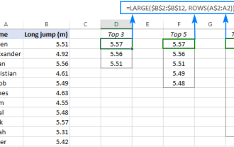
This tutorial demonstrates how to efficiently locate the top N values within a dataset and retrieve associated data using Excel formulas. Whether you need the highest, lowest, or those meeting specific criteria, this guide provides solutions. Findi
 Add a dropdown list to Outlook email template
Apr 01, 2025 am 05:13 AM
Add a dropdown list to Outlook email template
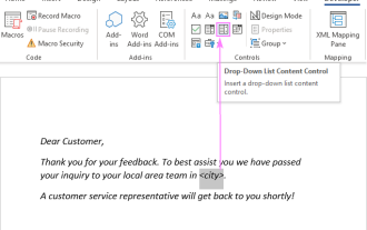
Apr 01, 2025 am 05:13 AM
This tutorial shows you how to add dropdown lists to your Outlook email templates, including multiple selections and database population. While Outlook doesn't directly support dropdowns, this guide provides creative workarounds. Email templates sav
 How to use Flash Fill in Excel with examples
Apr 05, 2025 am 09:15 AM
How to use Flash Fill in Excel with examples
Apr 05, 2025 am 09:15 AM
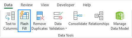
This tutorial provides a comprehensive guide to Excel's Flash Fill feature, a powerful tool for automating data entry tasks. It covers various aspects, from its definition and location to advanced usage and troubleshooting. Understanding Excel's Fla
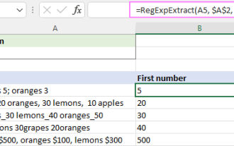 Regex to extract strings in Excel (one or all matches)
Mar 28, 2025 pm 12:19 PM
Regex to extract strings in Excel (one or all matches)
Mar 28, 2025 pm 12:19 PM
In this tutorial, you'll learn how to use regular expressions in Excel to find and extract substrings matching a given pattern. Microsoft Excel provides a number of functions to extract text from cells. Those functions can cope with most
 How to add calendar to Outlook: shared, Internet calendar, iCal file
Apr 03, 2025 am 09:06 AM
How to add calendar to Outlook: shared, Internet calendar, iCal file
Apr 03, 2025 am 09:06 AM
This article explains how to access and utilize shared calendars within the Outlook desktop application, including importing iCalendar files. Previously, we covered sharing your Outlook calendar. Now, let's explore how to view calendars shared with
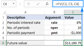 FV function in Excel to calculate future value
Apr 01, 2025 am 04:57 AM
FV function in Excel to calculate future value
Apr 01, 2025 am 04:57 AM
This tutorial explains how to use Excel's FV function to determine the future value of investments, encompassing both regular payments and lump-sum deposits. Effective financial planning hinges on understanding investment growth, and this guide prov
 MEDIAN formula in Excel - practical examples
Apr 11, 2025 pm 12:08 PM
MEDIAN formula in Excel - practical examples
Apr 11, 2025 pm 12:08 PM
This tutorial explains how to calculate the median of numerical data in Excel using the MEDIAN function. The median, a key measure of central tendency, identifies the middle value in a dataset, offering a more robust representation of central tenden
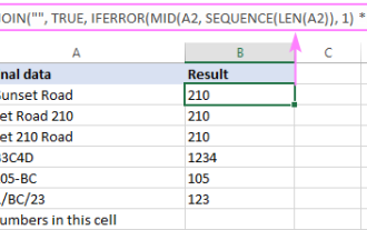 How to remove / split text and numbers in Excel cell
Apr 01, 2025 am 05:07 AM
How to remove / split text and numbers in Excel cell
Apr 01, 2025 am 05:07 AM
This tutorial demonstrates several methods for separating text and numbers within Excel cells, utilizing both built-in functions and custom VBA functions. You'll learn how to extract numbers while removing text, isolate text while discarding numbers
