

VLOOKUP in Google Sheets with formula examples

The tutorial explains the syntax of the Google Sheets VLOOKUP function and shows how to use Vlookup formulas for solving real-life tasks.
When working with interrelated data, one of the most common challenges is finding information across multiple sheets. You often perform such tasks in everyday life, for example when scanning a flight schedule board for your flight number to get the departing time and status. Google Sheets VLOOKUP works in a similar way - looks up and retrieves matching data from another table on the same sheet or from a different sheet.
A widespread opinion is that VLOOKUP is one of the most difficult and obscure functions. But that's not true! In fact, it's easy to do VLOOKUP in Google Sheets, and in a moment you will make sure of it.
Tip. For Microsoft Excel users, we have a separate Excel VLOOKUP tutorial with formula examples.
Google Sheets VLOOKUP - syntax and usage
The VLOOKUP function in Google Sheets is designed to perform a vertical lookup - search for a key value (unique identifier) down the first column in a specified range and return a value in the same row from another column.
The syntax for the Google Sheets VLOOKUP function is as follows:
VLOOKUP(search_key, range, index, [is_sorted])The first 3 arguments are required, the last one is optional:
Search_key - is the value to search for (lookup value or unique identifier). For example, you can search for the word "apple", number 10, or the value in cell A2.
Range - two or more columns of data for the search. The Google Sheets VLOOKUP function always searches in the first column of range.
Index - the column number in range from which a matching value (value in the same row as search_key) should be returned.
The first column in range has index 1. If index is less than 1, a Vlookup formula returns the #VALUE! error. If it's greater than the number of columns in range, VLOOKUP returns the #REF! error.
Is_sorted - indicates whether the lookup column is sorted (TRUE) or not (FALSE). In most cases, FALSE is recommended.
- If is_sorted is TRUE or omitted (default), the first column of range must be sorted in ascending order, i.e. from A to Z or from smallest to largest.
In this case a Vlookup formula returns an approximate match. More precisely, it searches for exact match first. If an exact match is not found, the formula searches for the closest match that is less than or equal to search_key. If all values in the lookup column are greater than the search key, an #N/A error is returned.
- If is_sorted is set to FALSE, no sorting is required. In this case, a Vlookup formula searches for exact match. If the lookup column contains 2 or more values exactly equal to search_key, the 1st value found is returned.
At first sight, the syntax may seem a bit complicated, but the below Google Sheet Vlookup formula example will make things easier to understand.
Supposing you have two tables: main table and lookup table like shown in the screenshot below. The tables have a common column (Order ID) that is a unique identifier. You aim to pull the status of each order from the lookup table to the main table.

Now, how do you use Google Sheets Vlookup to accomplish the task? To begin with, let's define the arguments for our Vlookup formula:
- Search_key - Order ID (A3), the value to be searched for in the first column of the Lookup table.
- Range - the Lookup table ($F$3:$G$14). Please pay attention that we lock the range by using absolute cell references since we plan to copy the formula to multiple cells.
- Index - 2 because the Status column from which we want to return a match is the 2nd column in range.
- Is_sorted - FALSE because our search column (F) is not sorted.
Putting all the arguments together, we get this formula:
=VLOOKUP(A3,$F$3:$G$14,2,false)
Enter it in the first cell (D3) of the main table, copy down the column, and you will get a result similar to this:

Is the Vlookup formula still difficult for you to comprehend? Then look at it this way:

5 things to know about Google Sheets VLOOKUP
As you already understood, the Google Sheets VLOOKUP function is a thing with nuances. Remembering these five simple facts will keep you out of trouble and help you avoid most common Vlookup errors.
- Google Sheets VLOOKUP cannot look at its left, it always searches in the first (leftmost) column of the range. To do a left Vlookup, use Google Sheets Index Match formula.
- Vlookup in Google Sheets is case-insensitive, meaning it does not distinguish lowercase and uppercase characters. For case-sensitive lookup, use this formula.
- If VLOOKUP returns incorrect results, set the is_sorted argument to FALSE to return exact matches. If this does not help, check other possible reasons why VLOOKUP fails.
- When is_sorted set to TRUE or omitted, remember to sort the first column of range in ascending order. In this case, the VLOOKUP function will use a faster binary search algorithm that correctly works only on sorted data.
- Google Sheets VLOOKUP can search with partial match based on the wildcard characters: the question mark (?) and asterisk (*). Please see this Vlookup formula example for more details.
How to use VLOOKUP in Google Sheets - formula examples
Now that you have a basic idea of how Google Sheets Vlookup works, it's time to try your hand in making a few formulas on your own. To make the below Vlookup examples easier to follow, you can open the sample Vlookup Google sheet.
How to Vlookup from a different sheet
In real-life spreadsheets, the main table and Lookup table often reside on different sheets. To refer your Vlookup formula to another sheet within the same spreadsheet, put the worksheet name followed by an exclamation mark (!) before the range reference. For example:
=VLOOKUP(A2,Sheet4!$A$2:$B$13,2,false)
The formula will search for the value in A2 in the range A2:A13 on Sheet4, and return a matching value from column B (2nd column in range).
If the sheet name includes spaces or non-alphabetical characters, be sure to enclose it in single quotation marks. For example:
=VLOOKUP(A2,'Lookup table'!$A$2:$B$13,2,false)

Tip. Instead of typing a reference to another sheet manually, you can have Google Sheets insert it for you automatically. For this, start typing your Vlookup formula and when it comes to the range argument, switch to the lookup sheet and select the range using a mouse. This will add a range reference to the formula, and you will only have to change a relative reference (default) to an absolute reference. To do this, either type the $ sign before the column letter and row number, or select the reference and press F4 to toggle between different reference types.
Google Sheets Vlookup with wildcard characters
In situations when you do not know the entire lookup value (search_key), but you do know a part of it, you can do a lookup with the following wildcard characters:
- Question mark (?) to match any single character, and
- Asterisk (*) to match any sequence of characters.
Let's say you want to retrieve information about a specific order from the table below. You cannot recall the order Id in full, but you remember that the first character is "A". So, you use an asterisk (*) to fill in the missing part, like this:
=VLOOKUP("a*",$A$2:$C$13,2,false)
Better yet, you can enter the known part of the search key in some cell and concatenate that cell with "*" to create a more versatile Vlookup formula:
To pull the item: =VLOOKUP($F$1&"*",$A$2:$C$13,2,false)
To pull the amount: =VLOOKUP($F$1&"*",$A$2:$C$13,3,false)

Tip. If you need to search for an actual question mark or asterisk character, put a tilde (~) before the character, e.g. "~*".
Google Sheets Index Match formula for left Vlookup
One of the most significant limitations of the VLOOKUP function (both in Excel and Google Sheets) is that it cannot look at its left. That is, if the search column is not the first column in the lookup table, Google Sheets Vlookup will fail. In such situations, use a more powerful and more durable Index Match formula:
INDEX (return_range, MATCH(search_key, lookup_range, 0))For example, to look up the A3 value (search_key) in G3:G14 (lookup_range) and return a match from F3:F14 (return_range), use this formula:
=INDEX($F$3:$F$14, MATCH (A3, $G$3:$G$14, 0))
The following screenshot shows this Index Match formula in action:

Another advantage of the Index Match formula compared to Vlookup is that it is immune to structural changes you make in the sheets since it references the return column directly. In particular, inserting or deleting a column in the lookup table breaks a Vlookup formula because the "hard-coded" index number becomes invalid, while the Index Match formula remains safe and sound.
For more information about INDEX MATCH, please see Why INDEX MATCH is a better alternative to VLOOKUP. Though the above tutorial targets Excel, INDEX MATCH in Google Sheets works exactly the same way, except for different names of the arguments.
Case-sensitive Vlookup in Google Sheets
In cases when the text case matters, use INDEX MATCH in combination with the TRUE and EXACT functions to make a case-sensitive Google Sheets Vlookup array formula:
ArrayFormula(INDEX(return_range, MATCH (TRUE,EXACT(lookup_range, search_key),0)))Assuming the search key is in cell A3, the lookup range is G3:G14 and the return range is F3:F14, the formula goes as follows:
=ArrayFormula(INDEX($F$3:$F$14, MATCH (TRUE,EXACT($G$3:$G$14, A3),0)))
As shown in the screenshot below, the formula has no problem with distinguishing uppercase and lowercase characters such as A-1001 and a-1001:

Tip. Pressing Ctrl Shift Enter while editing a formula inserts the ARRAYFORMULA function at the beginning of the formula automatically.
Vlookup formulas are the most common but not the only way to look up in Google Sheets. The next and the final section of this tutorial demonstrates an alternative.
Merge Sheets: formula-free alternative for Google Sheets Vlookup
If you are looking for a visual formula-free way to do Google spreadsheet Vlookup, consider using the Merge Sheets add-on. You can get it for free from the Google Sheets add-ons store:
Once the add-on is added to your Google Sheets, you can find it under the Extensions tab:

With the Merge Sheets add-on in place, you are ready to give it a field test. The source data is already familiar to you: we will be pulling information from the Status column based on the Order ID:

- Select any cell with data within the Main sheet and click Extensions > Merge Sheets > Start.
In most cases, the add-on will pick up the entire table for you automatically. If it doesn't, either click the Auto select button or select the range in your main sheet manually, and then click Next:

- Select the range in the Lookup sheet. The range does not necessarily have to be the same size as the range in the main sheet. In this example, the lookup table has 2 more rows than the main table.
- Select one or more key columns (unique identifiers) to compare. Since we are comparing the sheets by Order ID, we select only this column:
- Under Lookup columns, select the column(s) in the Lookup sheet from which you want to retrieve data. Under Main columns, choose the corresponding columns in the Main sheet into which you want to copy the data.
In this example, we are pulling information from the Status column on the Lookup sheet into the Status column on the Main sheet:
- Optionally, select one or more additional actions. Most often, you'd want to Add non-matching rows to the end of the main table, i.e. copy the rows that exist only in the lookup table to the end of the main table. And Update your main table right where it is:


Click Merge, allow the Merge Sheets add-on a moment for processing, and you are good to go!

Video: How to use Merge Sheets to vlookup without formulas
Vlookup multiple matches an easy way!
Filter & Extract Data is another Google Sheets tool for advanced lookup. The add-on can return all matches, not just the first one as the VLOOKUP function does. Moreover, it can evaluate multiple conditions, look up in any direction, and return all or the specified number of matches as values or formulas.
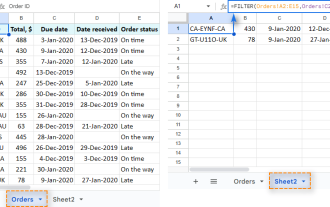
Remembering that a picture is worth a thousand words, let's see how the add-on works on real-life data. Supposing, some orders in our sample table contain several items, and you wish to retrieve all the items of a specific order. A Vlookup formula is unable to do this, while a more powerful QUERY function can. The problem is this function requires knowledge of the query language or at least SQL syntax. Have no desire to spend days studying this? Install the Filter & Extract Data add-on and get a flawless formula in seconds!
In your Google Sheet, click Extensions > Filter & Extract Data > Start, and define the lookup criteria:
- Select the range with your data (A1:D15).
- Specify how many matches to return (all in our case).
- Choose which columns to return the data from (Item, Amount and Status).
- Set one or more conditions. We want to pull the information about the order number input in F2, so we configure just one condition: Order ID = F2.
- Select the top-left cell for the result.
- Click Preview result to make sure you will get exactly what you are looking for.
- If all is good, click either Insert formula or Paste result.

For this example, we chose to return matches as formulas. So, you can now type any order number in F2, and the formula shown in the screenshot below will recalculate automatically:

To learn more about the add-on, visit the Filter & Extract Data home page or get it now from the Google Workspace Marketplace:
Video: How to vlookup multiple matches using the add-on
That's how you can do Google Sheets lookup. I thank you for reading and hope to see you on our blog next week!
Spreadsheet with formula examples
Sample Vlookup Spreadsheet
The above is the detailed content of VLOOKUP in Google Sheets with formula examples. For more information, please follow other related articles on the PHP Chinese website!
Hot AI Tools

Undresser.AI Undress
AI-powered app for creating realistic nude photos

AI Clothes Remover
Online AI tool for removing clothes from photos.

Undress AI Tool
Undress images for free

Clothoff.io
AI clothes remover

Video Face Swap
Swap faces in any video effortlessly with our completely free AI face swap tool!
Hot Article
Hot Tools

Notepad++7.3.1
Easy-to-use and free code editor

SublimeText3 Chinese version
Chinese version, very easy to use

Zend Studio 13.0.1
Powerful PHP integrated development environment

Dreamweaver CS6
Visual web development tools

SublimeText3 Mac version
God-level code editing software (SublimeText3)
Hot Topics


 How to add calendar to Outlook: shared, Internet calendar, iCal file
Apr 03, 2025 am 09:06 AM
How to add calendar to Outlook: shared, Internet calendar, iCal file
Apr 03, 2025 am 09:06 AM
This article explains how to access and utilize shared calendars within the Outlook desktop application, including importing iCalendar files. Previously, we covered sharing your Outlook calendar. Now, let's explore how to view calendars shared with
 How to use Flash Fill in Excel with examples
Apr 05, 2025 am 09:15 AM
How to use Flash Fill in Excel with examples
Apr 05, 2025 am 09:15 AM
This tutorial provides a comprehensive guide to Excel's Flash Fill feature, a powerful tool for automating data entry tasks. It covers various aspects, from its definition and location to advanced usage and troubleshooting. Understanding Excel's Fla
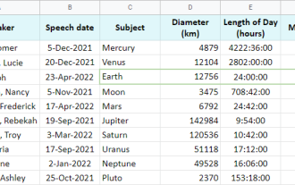
 MEDIAN formula in Excel - practical examples
Apr 11, 2025 pm 12:08 PM
MEDIAN formula in Excel - practical examples
Apr 11, 2025 pm 12:08 PM
This tutorial explains how to calculate the median of numerical data in Excel using the MEDIAN function. The median, a key measure of central tendency, identifies the middle value in a dataset, offering a more robust representation of central tenden
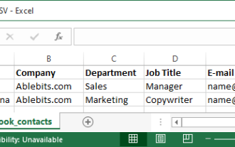 How to import contacts to Outlook (from CSV and PST file)
Apr 02, 2025 am 09:09 AM
How to import contacts to Outlook (from CSV and PST file)
Apr 02, 2025 am 09:09 AM
This tutorial demonstrates two methods for importing contacts into Outlook: using CSV and PST files, and also covers transferring contacts to Outlook Online. Whether you're consolidating data from an external source, migrating from another email pro
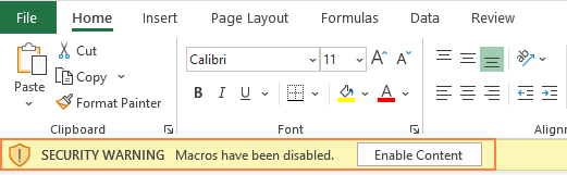 How to enable and disable macros in Excel
Apr 02, 2025 am 09:05 AM
How to enable and disable macros in Excel
Apr 02, 2025 am 09:05 AM
This article explores how to enable macros in Excel, covering macro security basics and safe VBA code execution. Macros, like any technology, have dual potential—beneficial automation or malicious use. Excel's default setting disables macros for sa
 How to use Google Sheets QUERY function – standard clauses and an alternative tool
Apr 02, 2025 am 09:21 AM
How to use Google Sheets QUERY function – standard clauses and an alternative tool
Apr 02, 2025 am 09:21 AM
This comprehensive guide unlocks the power of Google Sheets' QUERY function, often hailed as the most potent spreadsheet function. We'll dissect its syntax and explore its various clauses to master data manipulation. Understanding the Google Sheet
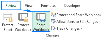 Excel shared workbook: How to share Excel file for multiple users
Apr 11, 2025 am 11:58 AM
Excel shared workbook: How to share Excel file for multiple users
Apr 11, 2025 am 11:58 AM
This tutorial provides a comprehensive guide to sharing Excel workbooks, covering various methods, access control, and conflict resolution. Modern Excel versions (2010, 2013, 2016, and later) simplify collaborative editing, eliminating the need to m
 How to use Google Sheets FILTER function
Apr 02, 2025 am 09:19 AM
How to use Google Sheets FILTER function
Apr 02, 2025 am 09:19 AM
Unlock the Power of Google Sheets' FILTER Function: A Comprehensive Guide Tired of basic Google Sheets filtering? This guide unveils the capabilities of the FILTER function, offering a powerful alternative to the standard filtering tool. We'll explo
