Are You Making These Mistakes in Classification Modeling?

Introduction

Assessing a machine learning model isn’t just the final step—it’s the keystone of success. Imagine building a cutting-edge model that dazzles with high accuracy, only to find it crumbles under real-world pressure. Evaluation is more than ticking off metrics; it’s about ensuring your model consistently performs in the wild. In this article, we’ll dive into the common pitfalls that can derail even the most promising classification models and reveal the best practices that can elevate your model from good to exceptional. Let’s turn your classification modeling tasks into reliable, effective solutions.

Overview

• Construct a classification model: Build a solid classification model with step-by-step guidance.
• Identify frequent mistakes: Spot and avoid common pitfalls in classification modeling.
• Comprehend overfitting: Understand overfitting and learn how to prevent it in your models.
• Improve model-building skills: Enhance your model-building skills with best practices and advanced techniques.

Table of contents

• Introduction
• Classification Modeling: An Overview
• Building a Basic Classification Model
  • 1. Data Preparation
  • 2. Logistic Regression
  • 3. Support Vector Machine (SVM)
  • 4. Decision Tree
  • 5. Neural Networks with TensorFlow
• Identifying the Mistakes
• Example of improved Logistic Regression using Grid Search
• Neural Networks with TensorFlow
• Understanding the Significance of Various Metrics
• Visualization of Model Performance
• Conclusion
• Frequently Asked Questions

Classification Modeling: An Overview

In the classification problem, we try to build a model that predicts the labels of the target variable using independent variables. As we deal with labeled target data, we’ll need supervised machine learning algorithms like Logistic Regression, SVM, Decision Tree, etc. We will also look at Neural Network models for solving the classification problem, identifying common mistakes people might make, and determining how to avoid them.

Building a Basic Classification Model

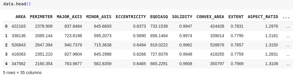
We’ll demonstrate creating a fundamental classification model using the Date-Fruit dataset from Kaggle. About the dataset: The target variable consists of seven types of date fruits: Barhee, Deglet Nour, Sukkary, Rotab Mozafati, Ruthana, Safawi, and Sagai. The dataset consists of 898 images of seven different date fruit varieties, and 34 features were extracted through image processing techniques. The objective is to classify these fruits based on their attributes.

1. Data Preparation

import pandas as pd

from sklearn.model_selection import train_test_split

from sklearn.preprocessing import StandardScaler

# Load the dataset

data = pd.read_excel('/content/Date_Fruit_Datasets.xlsx')

# Splitting the data into features and target

X = data.drop('Class', axis=1)

y = data['Class']

# Splitting the dataset into training and testing sets

X_train, X_test, y_train, y_test = train_test_split(X, y, test_size=0.3, random_state=42)

# Feature scaling

scaler = StandardScaler()

X_train = scaler.fit_transform(X_train)

X_test = scaler.transform(X_test)

2. Logistic Regression

from sklearn.linear_model import LogisticRegression

from sklearn.metrics import accuracy_score

# Logistic Regression Model

log_reg = LogisticRegression()

log_reg.fit(X_train, y_train)

# Predictions and Evaluation

y_train_pred = log_reg.predict(X_train)

y_test_pred = log_reg.predict(X_test)

# Accuracy

train_acc = accuracy_score(y_train, y_train_pred)

test_acc = accuracy_score(y_test, y_test_pred)

print(f'Logistic Regression - Train Accuracy: {train_acc}, Test Accuracy: {test_acc}')

Results:

- Logistic Regression - Train Accuracy: 0.9538<br><br>- Test Accuracy: 0.9222

Also read: An Introduction to Logistic Regression

3. Support Vector Machine (SVM)

from sklearn.svm import SVC

from sklearn.metrics import accuracy_score

# SVM

svm = SVC(kernel='linear', probability=True)

svm.fit(X_train, y_train)

# Predictions and Evaluation

y_train_pred = svm.predict(X_train)

y_test_pred = svm.predict(X_test)

train_accuracy = accuracy_score(y_train, y_train_pred)

test_accuracy = accuracy_score(y_test, y_test_pred)

print(f"SVM - Train Accuracy: {train_accuracy}, Test Accuracy: {test_accuracy}")

Results:

- SVM - Train Accuracy: 0.9602<br><br>- Test Accuracy: 0.9074

Also read: Guide on Support Vector Machine (SVM) Algorithm

4. Decision Tree

from sklearn.tree import DecisionTreeClassifier

from sklearn.metrics import accuracy_score

# Decision Tree

tree = DecisionTreeClassifier(random_state=42)

tree.fit(X_train, y_train)

# Predictions and Evaluation

y_train_pred = tree.predict(X_train)

y_test_pred = tree.predict(X_test)

train_accuracy = accuracy_score(y_train, y_train_pred)

test_accuracy = accuracy_score(y_test, y_test_pred)

print(f"Decision Tree - Train Accuracy: {train_accuracy}, Test Accuracy: {test_accuracy}")

Results:

- Decision Tree - Train Accuracy: 1.0000<br><br>- Test Accuracy: 0.8222

5. Neural Networks with TensorFlow

import numpy as np

from sklearn.preprocessing import LabelEncoder, StandardScaler

from sklearn.model_selection import train_test_split

from tensorflow.keras import models, layers

from tensorflow.keras.callbacks import EarlyStopping, ModelCheckpoint

# Label encode the target classes

label_encoder = LabelEncoder()

y_encoded = label_encoder.fit_transform(y)

# Train-test split

X_train, X_test, y_train, y_test = train_test_split(X, y_encoded, test_size=0.2, random_state=42)

# Feature scaling

scaler = StandardScaler()

X_train = scaler.fit_transform(X_train)

X_test = scaler.transform(X_test)

# Neural Network

model = models.Sequential([

layers.Dense(64, activation='relu', input_shape=(X_train.shape[1],)),

layers.Dense(32, activation='relu'),

layers.Dense(len(np.unique(y_encoded)), activation='softmax') # Ensure output layer size matches number of classes

])

model.compile(optimizer='adam', loss='sparse_categorical_crossentropy', metrics=['accuracy'])

# Callbacks

early_stopping = EarlyStopping(monitor='val_loss', patience=10, restore_best_weights=True)

model_checkpoint = ModelCheckpoint('best_model.keras', monitor='val_loss', save_best_only=True)

# Train the model

history = model.fit(X_train, y_train, epochs=100, batch_size=32, validation_data=(X_test, y_test),

callbacks=[early_stopping, model_checkpoint], verbose=1)

# Evaluate the model

train_loss, train_accuracy = model.evaluate(X_train, y_train, verbose=0)

test_loss, test_accuracy = model.evaluate(X_test, y_test, verbose=0)

print(f"Neural Network - Train Accuracy: {train_accuracy}, Test Accuracy: {test_accuracy}")

Results:

- Neural Network - Train Accuracy: 0.9234<br><br>- Test Accuracy: 0.9278

Also read: Build Your Neural Network Using Tensorflow

Identifying the Mistakes

Classification models can encounter several challenges that may compromise their effectiveness. It’s essential to recognize and tackle these problems to build reliable models. Below are some critical aspects to consider:

1. Overfitting and Underfitting:
   • Cross-Validation: Avoid depending solely on a single train-test split. Utilize k-fold cross-validation to better assess your model’s performance by testing it on various data segments.
   • Regularization: Highly complex models might overfit by capturing noise in the data. Regularization methods like pruning or regularisation should be used to penalize complexity.
   • Hyperparameter Optimization: Thoroughly explore and tune hyperparameters (e.g., through grid or random search) to balance bias and variance.
2. Ensemble Techniques:
   • Model Aggregation: Ensemble methods like Random Forests or Gradient Boosting combine predictions from multiple models, often resulting in enhanced generalization. These techniques can capture intricate patterns in the data while mitigating the risk of overfitting by averaging out individual model errors.
3. Class Imbalance:
   • Imbalanced Classes: In many cases one class might be less in count than others, leading to biased predictions. Methods like Oversampling, Undersampling or SMOTE must be used according to the problem.
4. Data Leakage:
   • Unintentional Leakage: Data leakage happens when information from outside the training set influences the model, causing inflated performance metrics. It’s crucial to ensure that the test data remains entirely unseen during training and that features derived from the target variable are managed with care.

Example of improved Logistic Regression using Grid Search

from sklearn.model_selection import GridSearchCV

# Implementing Grid Search for Logistic Regression

param_grid = {'C': [0.1, 1, 10, 100], 'solver': ['lbfgs']}

grid_search = GridSearchCV(LogisticRegression(multi_class='multinomial', max_iter=1000), param_grid, cv=5)

grid_search.fit(X_train, y_train)

# Best model

best_model = grid_search.best_estimator_

# Evaluate on test set

test_accuracy = best_model.score(X_test, y_test)

print(f"Best Logistic Regression - Test Accuracy: {test_accuracy}")

Results:

- Best Logistic Regression - Test Accuracy: 0.9611

Neural Networks with TensorFlow

Let’s focus on improving our previous neural network model, focusing on techniques to minimize overfitting and enhance generalization.

Early Stopping and Model Checkpointing

Early Stopping ceases training when the model’s validation performance plateaus, preventing overfitting by avoiding excessive learning from training data noise.

Model Checkpointing saves the model that performs best on the validation set throughout training, ensuring that the optimal model version is preserved even if subsequent training leads to overfitting.

import numpy as np

from sklearn.preprocessing import LabelEncoder, StandardScaler

from sklearn.model_selection import train_test_split

from tensorflow.keras import models, layers

from tensorflow.keras.callbacks import EarlyStopping, ModelCheckpoint

# Label encode the target classes

label_encoder = LabelEncoder()

y_encoded = label_encoder.fit_transform(y)

# Train-test split

X_train, X_test, y_train, y_test = train_test_split(X, y_encoded, test_size=0.2, random_state=42)

# Feature scaling

scaler = StandardScaler()

X_train = scaler.fit_transform(X_train)

X_test = scaler.transform(X_test)

# Neural Network

model = models.Sequential([

layers.Dense(64, activation='relu', input_shape=(X_train.shape[1],)),

layers.Dense(32, activation='relu'),

layers.Dense(len(np.unique(y_encoded)), activation='softmax') # Ensure output layer size matches number of classes

])

model.compile(optimizer='adam', loss='sparse_categorical_crossentropy', metrics=['accuracy'])

# Callbacks

early_stopping = EarlyStopping(monitor='val_loss', patience=10, restore_best_weights=True)

model_checkpoint = ModelCheckpoint('best_model.keras', monitor='val_loss', save_best_only=True)

# Train the model

history = model.fit(X_train, y_train, epochs=100, batch_size=32, validation_data=(X_test, y_test),

callbacks=[early_stopping, model_checkpoint], verbose=1)

# Evaluate the model

train_loss, train_accuracy = model.evaluate(X_train, y_train, verbose=0)

test_loss, test_accuracy = model.evaluate(X_test, y_test, verbose=0)

print(f"Neural Network - Train Accuracy: {train_accuracy}, Test Accuracy: {test_accuracy}")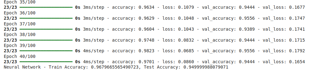

Understanding the Significance of Various Metrics

1. Accuracy: Although important, accuracy might not fully capture a model’s performance, particularly when dealing with imbalanced class distributions.
2. Loss: The loss function evaluates how well the predicted values align with the true labels; smaller loss values indicate higher accuracy.
3. Precision, Recall, and F1-Score: Precision evaluates the correctness of positive predictions, recall measures the model’s success in identifying all positive cases, and the F1-score balances precision and recall.
4. ROC-AUC: The ROC-AUC metric quantifies the model’s capacity to distinguish between classes regardless of the threshold setting.

from sklearn.metrics import classification_report, roc_auc_score

# Predictions

y_test_pred_proba = model.predict(X_test)

y_test_pred = np.argmax(y_test_pred_proba, axis=1)

# Classification report

print(classification_report(y_test, y_test_pred))

# ROC-AUC

roc_auc = roc_auc_score(y_test, y_test_pred_proba, multi_class='ovr')

print(f'ROC-AUC Score: {roc_auc}')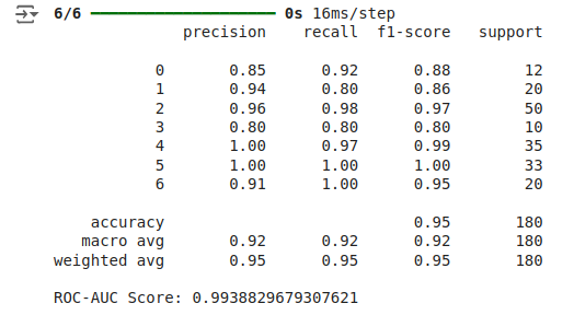

Visualization of Model Performance

The model’s performance during training can be seen by plotting learning curves for accuracy and loss, showing whether the model is overfitting or underfitting. We used early stopping to prevent overfitting, and this helps generalize to new data.

import matplotlib.pyplot as plt

# Plot training & validation accuracy values

plt.figure(figsize=(14, 5))

plt.subplot(1, 2, 1)

plt.plot(history.history['accuracy'])

plt.plot(history.history['val_accuracy'])

plt.title('Model Accuracy')

plt.xlabel('Epoch')

plt.ylabel('Accuracy')

plt.legend(['Train', 'Validation'], loc='upper left')

# Plot training & validation loss values

plt.subplot(1, 2, 2)

plt.plot(history.history['loss'])

plt.plot(history.history['val_loss'])

plt.title('Model Loss')

plt.xlabel('Epoch')

plt.ylabel('Loss')

plt.legend(['Train', 'Validation'], loc='upper left')

plt.show()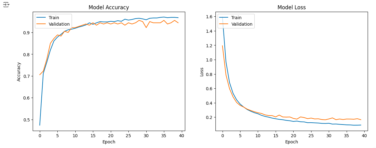

Conclusion

Meticulous evaluation is crucial to prevent issues like overfitting and underfitting. Building effective classification models involves more than choosing and training the right algorithm. Model consistency and reliability can be enhanced by implementing ensemble methods, regularization, tuning hyperparameters, and cross-validation. Although our small dataset may not have experienced significant overfitting, employing these methods ensures that models are robust and precise, leading to better decision-making in practical applications.

Frequently Asked Questions

Q1. Why is it important to assess a machine learning model beyond accuracy?

Ans. While accuracy is a key metric, it doesn’t always give a complete picture, especially with imbalanced datasets. Evaluating other aspects like consistency, robustness, and generalization ensures that the model performs well across various scenarios, not just in controlled test conditions.

Q2. What are the common mistakes to avoid when building classification models?

Ans. Common mistakes include overfitting, underfitting, data leakage, ignoring class imbalance, and failing to validate the model properly. These issues can lead to models that perform well in testing but fail in real-world applications.

Q3. How can I prevent overfitting in my classification model?

Ans. Overfitting can be mitigated through cross-validation, regularization, early stopping, and ensemble methods. These approaches help balance the model’s complexity and ensure it generalizes well to new data.

Q4. What metrics should I use to evaluate the performance of my classification model?

Ans. Beyond accuracy, consider metrics like precision, recall, F1-score, ROC-AUC, and loss. These metrics provide a more nuanced understanding of the model’s performance, especially in handling imbalanced data and making accurate predictions.

The above is the detailed content of Are You Making These Mistakes in Classification Modeling?. For more information, please follow other related articles on the PHP Chinese website!