Detailed introduction to python machine learning decision tree

Decision Trees (DTs) are an unsupervised learning method used for classification and regression.

Advantages: The computational complexity is not high, the output results are easy to understand, insensitive to missing intermediate values, and can handle irrelevant feature data
Disadvantages: Over-matching may occur
ApplicableData type: Numerical and nominal source code download https://www.manning.com/books/machine-learning-in-action

Run demo

Key algorithm

if so return Class tag;

else

Find the best features to divide the dataset ##createBranch and add the return result to the branch node
return branch node

Corresponding codedef createTree(dataSet,labels):
　class
List

= [example[-1] for example in dataSet] is not dataset[-1] {the last element of the dataset}, but at this time, the first element from the last in each element of the dataset

if classList.

count

(classList[0]) == len(classList): If the returned classified List count type is the same, then return this type! Whether it can be classified at the sub -node. If you return it, other types will be ceded
在 在 在 在 在 在 在 Return classList [0] #Stop Splitting When all of the classs are iF Len (dataSet [0]) == 1: #stop splitting when there are no more features in dataSet If there is only one element Return majorityCnt(classList) bestFeat = chooseBestFeatureToSplit(dataSet) BestFeatLabel = labels[bestFeat ]   And get this label flippers or no surfaces?
  myTree = {bestFeatLabel:{}}   Then create a subtree of the best category   del(labels[bestFeat])   Delete the best category featValues ​​= [example[bestFeat] for example in dataSet] uniqueVals = set(featValues) set is a classification, see how many types there are for value in uniqueVals:
subLabels = labels[:] #copy all of labels, so trees do mess up existing labels
MyTree [Bestfeatlabel] [Value] = Createtree (SPLITDATASET (DataSET, Bestfeat, Value), Sublabels)
rn mytree

is dividing data The change in information before and after a set is called information gain. The biggest principle for dividing a data set is to make disordered data more orderly. This is understood as the pie-cutting principle:




# Use unit entropy to describe the complexity and amount of information. Corresponding to the density of the cake, if it is a vertically cut cake of equal density,

The weight of each part g = total G * its proportion in the great circle! Analogously, if the information entropy is the same after partitioning, the small h of each small part of the data = pro * total H, and the sum h[i] = H.

However: what we need is just the opposite: what is needed It's not that the information entropy is the same, but it's unequal. For example, the green ones may be grass fillings, the yellow ones are apple fillings, and the blue ones are purple sweet potatoes. Each one has a different density!

We need to divide it correctly! Sort it out and find the line that approximates the different fillings. The small h here will be minimized, and eventually the total H will approach the minimum value while the area remains unchanged, which is an optimization problem to solve.

DebuggingProcess
calcShannonEnt : [[1, 'no'], [1, 'no']] = 0 log(1, 2) * 0.4 = 0 Why is it 0, because pro must be 1
log(prob,2) log(1,2) = 0;2^0=1, because prob : [[1, 'yes'], [1, 'yes'], [0, 'no']] = 0.91 >> * 0.6 = 0.55
25 lines for featVec in dataSet: Frequency counting for prop
chooseBestFeatureToSplit()　
0.9709505944546686 = calcShannonEnt(dataSet) : [[1, 1, 'yes' ], [1, 1, 'yes'], [1, 0, 'no'], [0, 1, 'no'], [0, 1, 'no']]

#Detection Whether each sub-item of the data set belongs to the same category: If the values ​​are all a, and the results are all y or n, it is a category. Therefore, just two parameter inputs
0.5509775004326937 = += prob * calcShannonEnt(subDataSet) separated After subsetting, the probability * Shannon drop is obtained, and the original overall Shannon drop ratio is

# 数据越接近，香浓熵值越少，越接近0 ，越不同，越多分逻辑，香浓熵就越大
# 只计算 其dataSet的featVec[-1] 结果标签
def calcShannonEnt(dataSet):

0.4199730940219749 infoGain = baseEntropy - newEntropy

Summary: 　

At first, I couldn’t understand the code and didn’t understand what it was supposed to do! Classification, our goal is to classify a bunch of data and label it with labels.
Like k-nearby classify([0, 0], group, labels, 3), it means that the new data [0,0] is classified in the group, labels data according to the k=3 neighbor algorithm! Group corresponds to label!

I saw

later. , result label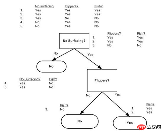

So, we need to cut out each dimension + result label into a two-dimensional array to compare and classify

The test should be to divide the first n dimensions Value, vector input, output is yes or no!

It seems dizzy at first, but it is clearer. It is easier to understand after straightening out your ideas and looking at the code!

After understanding the target and initial data, you understand that classList is the result label! , is the corresponding result label

corresponding to the dataset to be classified, and labels is the feature name, corresponding to the dimension of the starting dataset, the name of the feature strname
bestFeatLabel is the dimension name of the best classification feature, whether it is the first dimension or the second dimension , the N
featValues ​​is the value array under the dimension of bestFeatLabel. It is the groups under this dimension that are used to make new classification comparisons.
uniqueVals uses set to determine whether it is of the same type,
For example
DataSet = [[1, 1, 'yes'],[0, 1, 'yes'],[1, 0, 'no' ],[1, 0, 'no'],[0, 0, 'no']]
Labels = ['no surfacing','flippers',]
createTree like this:{'flippers': {0: 'no', 1: 'yes'}} directly omits the dimension of no surfacing





Finally, let me use a paragraph to talk about decision-making Tree:

The essence of a decision tree is to speed up efficiency! Use 'maximum optimal' to divide the first negative label, and the positive label should continue to be divided! And if negative, directly return the leaf node answer! The corresponding other dimensions will not continue to be judged!

Theoretically, even if you don’t use the decision tree algorithm, you can blindly exhaust all the data, that is, go through all the dimensions of the data every time! And there is the last label answer! Number of dimensions * number of data! For complexity! This is the matching answer to memory! Suitable expert system! Poor ability to predict situations that do not occur! But the data volume is large, the speed is fast, and it can also feel intelligent! Because it is a repeat of past experience! But is it dead? No, it's not dead! Exhaustion is dead, but decision trees are dynamic! educational! Change tree! At least it's built to be dynamic! When data is incomplete, it can also be incomplete! When a judgment can be solved, use one judgment, and if it cannot, then another one is needed! Dimensions increased!

The above is the detailed content of Detailed introduction to python machine learning decision tree. For more information, please follow other related articles on the PHP Chinese website!