Basic operations of DataFrame introduced by pandas library

How to delete list hollow characters?
The simplest method: new_list = [ x for x in li if x != '' ]

---

Today is May 1st.

This part mainly studies the basic operations in pandas based on the previous two data structures.

设有DataFrame结果的数据a如下所示：    
       a  b  c
one    4  1  1
two    6  2  0
three  6  1  6

---

1. View data (the method of viewing object is also applicable to Series)

1. View the xx rows before or after the DataFrame Line xx
a=DataFrame(data);
a.head(6) means displaying the first 6 rows of data. If there are no parameters in head(), all data will be displayed. .
a.tail(6) means displaying the last 6 rows of data. If there are no parameters in tail(), all data will be displayed.

2. View the index, columns and values ​​of the DataFrame
a.index; a.columns; a.values

3.describe ()FunctionFor fast statistical summary of data
a.describe() performs statistics on each column of data, including count, mean, std, each quantile, etc.

4. Transpose the data
a.T

5. Sort the axis
a.sort _index(axis=1,ascending=False);
axis=1 means to sort all columns, and the following numbers will also move accordingly . The following ascending=False means to sort in descending order, and the default is ascending order when the parameter is missing.

6. Sort the values ​​in the DataFrame
a.sort(columns='x')
That is, sort the x column in a from small to large . Note that it is only the x column, and the above sorting by axis will operate on all columns.

2. Select the object

1. Select the data of specific columns and rows
a['x'] Then the column whose columns is x will be returned. Note that this method can only return one column at a time. a.x has the same meaning as a['x'].

Get the row data and select it by slicing []
For example: a[0:3] will return the data of the first three rows.

2.loc selects data through labels
a.loc['one'] will default to selecting the behavior 'one' row;

a.loc[:,['a','b'] ] means selecting all rows and columns whose columns are a and b;

a.loc[['one' ,'two'],['a','b']] means selecting the two rows 'one' and 'two' and the columns whose columns are a and b;

a.loc['one' ,'a'] has the same effect as a.loc[['one'],['a']], but the former only displays the corresponding value, while the latter displays the corresponding row and column labels.

3.iloc selects data directly through position
This is similar to selecting through tags
a.iloc[1:2,1:2] will be displayed The data in the first row and the first column; (the value after the slice cannot be obtained)

a.iloc[1:2] That is, when there is no value in the subsequent column, the row position is selected as 1 by default The data;

a.iloc[[0,2],[1,2]] means you can freely select the data corresponding to the row position and column position.

4. Use conditions to select
Use separate columns to select data
a[a.c>0] means selecting column c Data greater than 0

Use where to select data
a[a>0] table directly selects all data greater than 0 in a

Use isin() to select specific Rows containing a specific value in column
a1=a.copy()
a1[a1['one'].isin(['2','3']) ] The table displays all rows that meet the condition: the value in column one contains '2', '3'.

3. Setting value (assignment)

The assignment operation can be done directly based on the above selection operation.
Example a.loc[:,['a','c']]=9 will set the values ​​in all rows of columns a and c to 9
a.iloc[:,[1,3] ]=9 also means to set the values ​​in all rows of columns a and c to 9

At the same time, you can still use conditions to assign values ​​directly
a[a>0]=-a means to set the value in a All numbers greater than 0 are converted to negative values

4. Missing value processing

In pandas, use np.nan to replace missing values. These values ​​will not be included in the calculation by default.

1.reindex() method
is used to change/add/delete the index on the specified axis , this A copy of the original data will be returned.
a.reindex(index=list(a.index)+['five'],columns=list(a.columns)+['d'])

a.reindex(index=['one','five'],columns=list(a.columns)+['d'])

即用index=[]表示对index进行操作，columns表对列进行操作。

2.对缺失值进行填充
a.fillna(value=x)
表示用值为x的数来对缺失值进行填充

3.去掉包含缺失值的行
a.dropna(how='any')
表示去掉所有包含缺失值的行

五、合并

1.contact
contact(a1,axis=0/1，keys=['xx','xx','xx',...])，其中a1表示要进行进行连接的列表数据,axis=1时表横着对数据进行连接。axis=0或不指定时，表将数据竖着进行连接。a1中要连接的数据有几个则对应几个keys，设置keys是为了在数据连接以后区分每一个原始a1中的数据。

例：a1=[b['a'],b['c']]
result=pd.concat(a1,axis=1，keys=['1','2'])

2.Append 将一行或多行数据连接到一个DataFrame上
a.append(a[2:],ignore_index=True)
表示将a中的第三行以后的数据全部添加到a中，若不指定ignore_index参数，则会把添加的数据的index保留下来，若ignore_index=Ture则会对所有的行重新自动建立索引。

3.merge类似于SQL中的join
设a1,a2为两个dataframe,二者中存在相同的键值，两个对象连接的方式有下面几种：
(1)内连接，pd.merge(a1, a2, on='key')
(2)左连接，pd.merge(a1, a2, on='key', how='left')
(3)右连接，pd.merge(a1, a2, on='key', how='right')
(4)外连接， pd.merge(a1, a2, on='key', how='outer')
至于四者的具体差别，具体学习参考sql中相应的语法。

六、分组（groupby）

用pd.date_range函数生成连续指定天数的的日期
pd.date_range('20000101',periods=10)

def shuju():
    data={
        'date':pd.date_range('20000101',periods=10),
        'gender':np.random.randint(0,2,size=10),
        'height':np.random.randint(40,50,size=10),
        'weight':np.random.randint(150,180,size=10)
    }
a=DataFrame(data)
print(a)
        date  gender  height  weight
0 2000-01-01       0      47     165
1 2000-01-02       0      46     179
2 2000-01-03       1      48     172
3 2000-01-04       0      45     173
4 2000-01-05       1      47     151
5 2000-01-06       0      45     172
6 2000-01-07       0      48     167
7 2000-01-08       0      45     157
8 2000-01-09       1      42     157
9 2000-01-10       1      42     164

用a.groupby('gender').sum()得到的结果为：  #注意在python中groupby(''xx)后要加sum()，不然显示
不了数据对象。
gender     height  weight               
0           256     989
1           170     643

此外用a.groupby('gender').size()可以对各个gender下的数目进行计数。

所以可以看到groupby的作用相当于：
按gender对gender进行分类，对应为数字的列会自动求和，而为字符串类型的列则不显示；当然也可以同时groupby(['x1','x2',...])多个字段，其作用与上面类似。

七、Categorical按某一列重新编码分类

如六中要对a中的gender进行重新编码分类，将对应的0，1转化为male，female，过程如下：

a['gender1']=a['gender'].astype('category')
a['gender1'].cat.categories=['male','female']  #即将0，1先转化为category类型再进行编码。

 print(a)得到的结果为：
      date    gender  height  weight gender1
0 2000-01-01       1      40     163  female
1 2000-01-02       0      44     177    male
2 2000-01-03       1      40     167  female
3 2000-01-04       0      41     161    male
4 2000-01-05       0      48     177    male
5 2000-01-06       1      46     179  female
6 2000-01-07       1      42     154  female
7 2000-01-08       1      43     170  female
8 2000-01-09       0      46     158    male
9 2000-01-10       1      44     168  female

所以可以看出重新编码后的编码会自动增加到dataframe最后作为一列。

八、相关操作

描述性统计：
1.a.mean()  默认对每一列的数据求平均值；若加上参数a.mean(1)则对每一行求平均值；

2.统计某一列x中各个值出现的次数：a['x'].value_counts()；

3.对数据应用函数
a.apply(lambda x:x.max()-x.min())
表示返回所有列中最大值-最小值的差。

4.字符串相关操作
a['gender1'].str.lower()  将gender1中所有的英文大写转化为小写，注意dataframe没有str属性，只有series有，所以要选取a中的gender1字段。

九、时间序列

在六中用pd.date_range('xxxx',periods=xx,freq='D/M/Y....')函数生成连续指定天数的的日期列表。
例如pd.date_range('20000101',periods=10),其中periods表示持续频数；
pd.date_range('20000201','20000210',freq='D')也可以不指定频数，只指定起始日期。

此外如果不指定freq，则默认从起始日期开始，频率为day。其他频率表示如下：

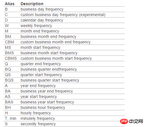
1.png

十、画图(plot)

在pycharm中首先要：import matplotlib.pyplot as plt
a=Series(np.random.randn(1000),index=pd.date_range('20100101',periods=1000))
b=a.cumsum()
b.plot()
plt.show()    #最后一定要加这个plt.show()，不然不会显示出图来。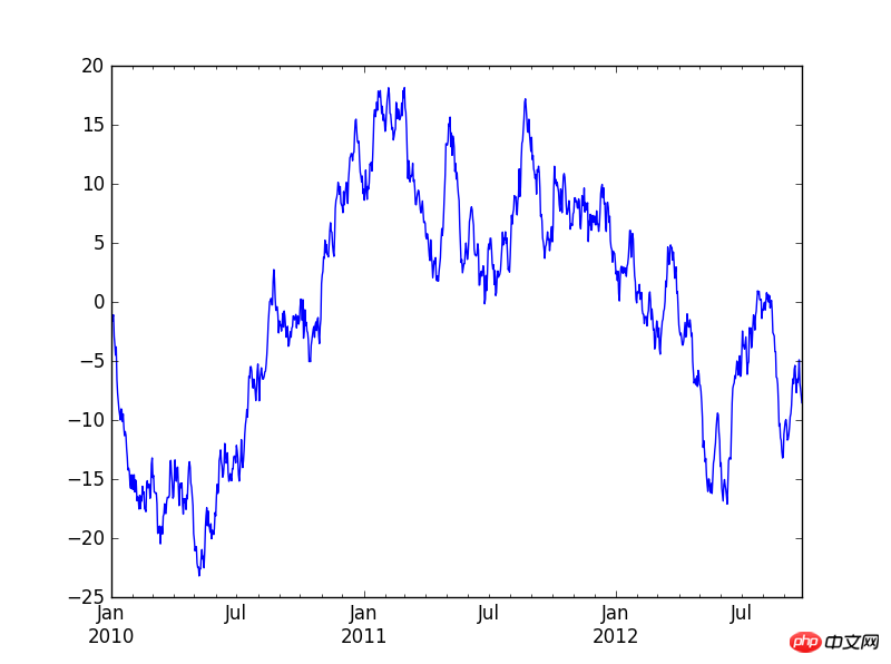

2.PNG

也可以使用下面的代码来生成多条时间序列图：

a=DataFrame(np.random.randn(1000，4),index=pd.date_range('20100101',periods=1000),columns=list('ABCD'))
b=a.cumsum()
b.plot()
plt.show()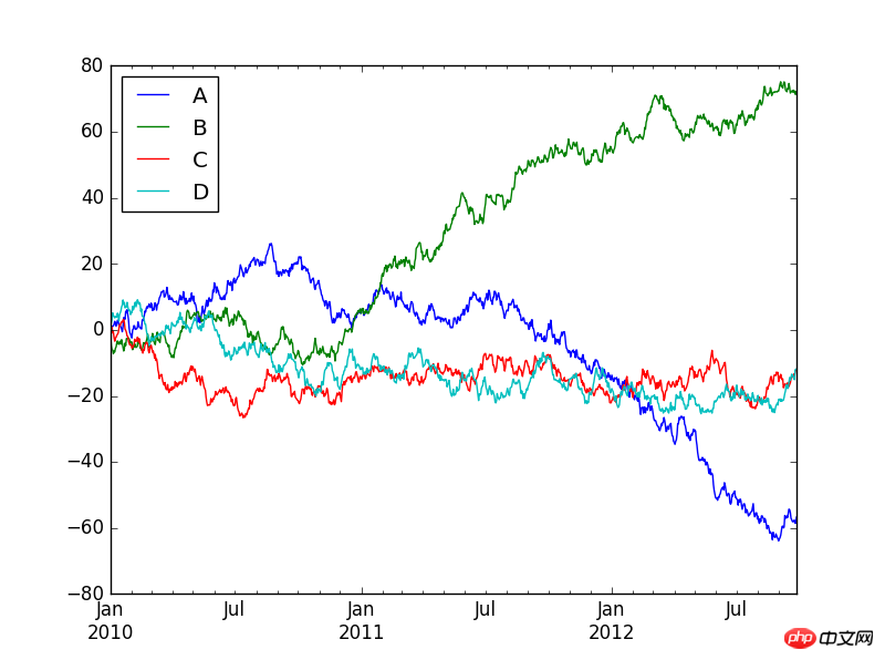

3.png

十一、导入和导出文件

写入和读取excel文件
虽然写入excel表时有两种写入xls和csv，但建议少使用csv，不然在表中调整数据格式时，保存时一直询问你是否保存新格式，很麻烦。而在读取数据时，如果指定了哪一张sheet，则在pycharm又会出现格式不对齐。

还有将数据写入表格中时，excel会自动给你在表格最前面增加一个字段，对数据行进行编号。

a.to_excel(r'C:\\Users\\guohuaiqi\\Desktop\\2.xls',sheet_name='Sheet1')    

a=pd.read_excel(r'C:\\Users\\guohuaiqi\\Desktop\\2.xls','Sheet1',na_values=['NA'])

注意sheet_name后面的Sheet1中的首字母大写；读取数据时，可以指定读取哪一张表中的数据，而
且对缺失值补上NA。

最后再附上写入和读取csv格式的代码：
a.to_csv(r'C:\\Users\\guohuaiqi\\Desktop\\1.csv'，sheet_name='Sheet1')
a=pd.read_csv(r'C:\\Users\\guohuaiqi\\Desktop\\1.csv',na_values=['NA'])

       

The above is the detailed content of Basic operations of DataFrame introduced by pandas library. For more information, please follow other related articles on the PHP Chinese website!