Python digital image processing skeleton extraction and watershed algorithm

This article mainly introduces the skeleton extraction and watershed algorithm of python digital image processing. Now I will share it with you and give you a reference. Let’s take a look together

Skeleton extraction and watershed algorithm also belong to the category of morphological processing, and are placed in the morphology sub-module.

1. Skeleton extraction

Skeleton extraction, also called binary image thinning. This algorithm can refine a connected region into a width of one pixel for feature extraction and target topology representation.

The morphology submodule provides two functions for skeleton extraction, namely the Skeletonize() function and the medial_axis() function. Let’s look at the Skeletonize() function first.

The format is: skimage.morphology.skeletonize(image)

The input and output are both binary images.

Example 1:

from skimage import morphology,draw
import numpy as np
import matplotlib.pyplot as plt
#创建一个二值图像用于测试
image = np.zeros((400, 400))
#生成目标对象1(白色U型)
image[10:-10, 10:100] = 1
image[-100:-10, 10:-10] = 1
image[10:-10, -100:-10] = 1
#生成目标对象2（X型）
rs, cs = draw.line(250, 150, 10, 280)
for i in range(10):
 image[rs + i, cs] = 1
rs, cs = draw.line(10, 150, 250, 280)
for i in range(20):
 image[rs + i, cs] = 1
#生成目标对象3（O型）
ir, ic = np.indices(image.shape)
circle1 = (ic - 135)**2 + (ir - 150)**2 < 30**2
circle2 = (ic - 135)**2 + (ir - 150)**2 < 20**2
image[circle1] = 1
image[circle2] = 0

#实施骨架算法
skeleton =morphology.skeletonize(image)

#显示结果
fig, (ax1, ax2) = plt.subplots(nrows=1, ncols=2, figsize=(8, 4))
ax1.imshow(image, cmap=plt.cm.gray)
ax1.axis('off')
ax1.set_title('original', fontsize=20)
ax2.imshow(skeleton, cmap=plt.cm.gray)
ax2.axis('off')
ax2.set_title('skeleton', fontsize=20)
fig.tight_layout()
plt.show()

Generate a test image with three target objects on it, and perform skeleton extraction respectively. The results are as follows:

Example 2: Using the system’s own horse pictures for skeleton extraction

from skimage import morphology,data,color
import matplotlib.pyplot as plt
image=color.rgb2gray(data.horse())
image=1-image #反相
#实施骨架算法
skeleton =morphology.skeletonize(image)
#显示结果
fig, (ax1, ax2) = plt.subplots(nrows=1, ncols=2, figsize=(8, 4))

ax1.imshow(image, cmap=plt.cm.gray)
ax1.axis('off')
ax1.set_title('original', fontsize=20)
ax2.imshow(skeleton, cmap=plt.cm.gray)
ax2.axis('off')
ax2.set_title('skeleton', fontsize=20)
fig.tight_layout()
plt.show()

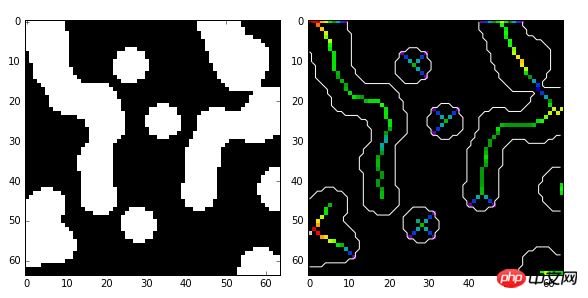
medial_axis means the central axis. The medial axis transformation method is used to calculate the width of the foreground (1 value) target object. The format is:

skimage.morphology.medial_axis (image,mask=None,return_distance=False)

mask: mask. The default is None. If a mask is given, the skeleton algorithm will be performed only on the pixel values ​​within the mask.

return_distance: bool value, default is False. If it is True, in addition to returning the skeleton, the distance transformation value will also be returned at the same time. The distance here refers to the distance between all points on the central axis and the background point.

import numpy as np
import scipy.ndimage as ndi
from skimage import morphology
import matplotlib.pyplot as plt
#编写一个函数，生成测试图像
def microstructure(l=256):
 n = 5
 x, y = np.ogrid[0:l, 0:l]
 mask = np.zeros((l, l))
 generator = np.random.RandomState(1)
 points = l * generator.rand(2, n**2)
 mask[(points[0]).astype(np.int), (points[1]).astype(np.int)] = 1
 mask = ndi.gaussian_filter(mask, sigma=l/(4.*n))
 return mask > mask.mean()
data = microstructure(l=64) #生成测试图像

#计算中轴和距离变换值
skel, distance =morphology.medial_axis(data, return_distance=True)
#中轴上的点到背景像素点的距离
dist_on_skel = distance * skel
fig, (ax1, ax2) = plt.subplots(1, 2, figsize=(8, 4))
ax1.imshow(data, cmap=plt.cm.gray, interpolation='nearest')
#用光谱色显示中轴
ax2.imshow(dist_on_skel, cmap=plt.cm.spectral, interpolation='nearest')
ax2.contour(data, [0.5], colors='w') #显示轮廓线
fig.tight_layout()
plt.show()

2. Watershed algorithm

A watershed refers to a ridge in geography, and water usually flows along both sides of the ridge to different "catchment basins." The watershed algorithm is a classic algorithm for image segmentation and a mathematical morphological segmentation method based on topology theory. If the target objects in the image are connected together, it will be more difficult to segment. The watershed algorithm is often used to deal with such problems and usually achieves better results.

The watershed algorithm can be combined with distance transformation to find the "catchment basin" and "watershed boundary" to segment the image. The distance transformation of a binary image is the distance from each pixel to the nearest non-zero pixel. We can use the scipy package to calculate the distance transformation.

In the example below, two overlapping circles need to be separated. We first calculate the distance transformation from these white pixels on the circle to the black background pixels, select the maximum value in the distance transformation as the initial marker point (if it is an inverted color, take the minimum value), starting from these marker points The two catchment basins get bigger and bigger, and finally intersect at the mountain ridge. Disconnected from the mountain ridge, we get two separate circles.

Example 1: Mountain ridge image segmentation based on distance transform

import numpy as np
import matplotlib.pyplot as plt
from scipy import ndimage as ndi
from skimage import morphology,feature
#创建两个带有重叠圆的图像
x, y = np.indices((80, 80))
x1, y1, x2, y2 = 28, 28, 44, 52
r1, r2 = 16, 20
mask_circle1 = (x - x1)**2 + (y - y1)**2 < r1**2
mask_circle2 = (x - x2)**2 + (y - y2)**2 < r2**2
image = np.logical_or(mask_circle1, mask_circle2)
#现在我们用分水岭算法分离两个圆
distance = ndi.distance_transform_edt(image) #距离变换
local_maxi =feature.peak_local_max(distance, indices=False, footprint=np.ones((3, 3)),
       labels=image) #寻找峰值
markers = ndi.label(local_maxi)[0] #初始标记点
labels =morphology.watershed(-distance, markers, mask=image) #基于距离变换的分水岭算法
fig, axes = plt.subplots(nrows=2, ncols=2, figsize=(8, 8))
axes = axes.ravel()
ax0, ax1, ax2, ax3 = axes
ax0.imshow(image, cmap=plt.cm.gray, interpolation='nearest')
ax0.set_title("Original")
ax1.imshow(-distance, cmap=plt.cm.jet, interpolation='nearest')
ax1.set_title("Distance")
ax2.imshow(markers, cmap=plt.cm.spectral, interpolation='nearest')
ax2.set_title("Markers")
ax3.imshow(labels, cmap=plt.cm.spectral, interpolation='nearest')
ax3.set_title("Segmented")
for ax in axes:
 ax.axis('off')
fig.tight_layout()
plt.show()

The watershed algorithm can also be used with Gradient is combined to achieve image segmentation. Generally, gradient images have higher pixel values ​​at the edges and lower pixel values ​​elsewhere. Ideally, the ridges should be exactly at the edges. Therefore, we can find ridges based on gradients.

Example 2: Gradient-based watershed image segmentation

import matplotlib.pyplot as plt
from scipy import ndimage as ndi
from skimage import morphology,color,data,filter
image =color.rgb2gray(data.camera())
denoised = filter.rank.median(image, morphology.disk(2)) #过滤噪声
#将梯度值低于10的作为开始标记点
markers = filter.rank.gradient(denoised, morphology.disk(5)) <10
markers = ndi.label(markers)[0]
gradient = filter.rank.gradient(denoised, morphology.disk(2)) #计算梯度
labels =morphology.watershed(gradient, markers, mask=image) #基于梯度的分水岭算法
fig, axes = plt.subplots(nrows=2, ncols=2, figsize=(6, 6))
axes = axes.ravel()
ax0, ax1, ax2, ax3 = axes
ax0.imshow(image, cmap=plt.cm.gray, interpolation='nearest')
ax0.set_title("Original")
ax1.imshow(gradient, cmap=plt.cm.spectral, interpolation='nearest')
ax1.set_title("Gradient")
ax2.imshow(markers, cmap=plt.cm.spectral, interpolation='nearest')
ax2.set_title("Markers")
ax3.imshow(labels, cmap=plt.cm.spectral, interpolation='nearest')
ax3.set_title("Segmented")
for ax in axes:
 ax.axis('off')
fig.tight_layout()
plt.show()

Related recommendations:

Advanced morphological processing of python digital image processing

The above is the detailed content of Python digital image processing skeleton extraction and watershed algorithm. For more information, please follow other related articles on the PHP Chinese website!