 Backend Development
 Python Tutorial
 How TensorFlow implements random training and batch training
How TensorFlow implements random training and batch training
This article mainly introduces the method of TensorFlow to implement random training and batch training. Now I will share it with you and give you a reference. Let’s take a look together
TensorFlow updates model variables. It can operate on one data point at a time or on large amounts of data at once. Operating on a single training example can lead to a "quirky" learning process, but training with large batches can be computationally expensive. Which type of training is chosen is very critical to the convergence of the machine learning algorithm.
In order for TensorFlow to calculate variable gradients for backpropagation to work, we must measure the loss on one or more samples.
Random training will randomly sample pairs of training data and target data to complete the training. Another option is to average the loss for gradient calculation in a large batch training, and the batch training size can be expanded to the entire data set at once. Here we show how to extend the previous example of a regression algorithm - using random training and batch training.
Batch training and random training differ in their optimizer methods and convergence.
# 随机训练和批量训练
#----------------------------------
#
# This python function illustrates two different training methods:
# batch and stochastic training. For each model, we will use
# a regression model that predicts one model variable.
import matplotlib.pyplot as plt
import numpy as np
import tensorflow as tf
from tensorflow.python.framework import ops
ops.reset_default_graph()
# 随机训练:
# Create graph
sess = tf.Session()
# 声明数据
x_vals = np.random.normal(1, 0.1, 100)
y_vals = np.repeat(10., 100)
x_data = tf.placeholder(shape=[1], dtype=tf.float32)
y_target = tf.placeholder(shape=[1], dtype=tf.float32)
# 声明变量 (one model parameter = A)
A = tf.Variable(tf.random_normal(shape=[1]))
# 增加操作到图
my_output = tf.multiply(x_data, A)
# 增加L2损失函数
loss = tf.square(my_output - y_target)
# 初始化变量
init = tf.global_variables_initializer()
sess.run(init)
# 声明优化器
my_opt = tf.train.GradientDescentOptimizer(0.02)
train_step = my_opt.minimize(loss)
loss_stochastic = []
# 运行迭代
for i in range(100):
 rand_index = np.random.choice(100)
 rand_x = [x_vals[rand_index]]
 rand_y = [y_vals[rand_index]]
 sess.run(train_step, feed_dict={x_data: rand_x, y_target: rand_y})
 if (i+1)%5==0:
  print('Step #' + str(i+1) + ' A = ' + str(sess.run(A)))
  temp_loss = sess.run(loss, feed_dict={x_data: rand_x, y_target: rand_y})
  print('Loss = ' + str(temp_loss))
  loss_stochastic.append(temp_loss)
# 批量训练:
# 重置计算图
ops.reset_default_graph()
sess = tf.Session()

# 声明批量大小
# 批量大小是指通过计算图一次传入多少训练数据
batch_size = 20

# 声明模型的数据、占位符
x_vals = np.random.normal(1, 0.1, 100)
y_vals = np.repeat(10., 100)
x_data = tf.placeholder(shape=[None, 1], dtype=tf.float32)
y_target = tf.placeholder(shape=[None, 1], dtype=tf.float32)

# 声明变量 (one model parameter = A)
A = tf.Variable(tf.random_normal(shape=[1,1]))

# 增加矩阵乘法操作(矩阵乘法不满足交换律)
my_output = tf.matmul(x_data, A)

# 增加损失函数
# 批量训练时损失函数是每个数据点L2损失的平均值
loss = tf.reduce_mean(tf.square(my_output - y_target))

# 初始化变量
init = tf.global_variables_initializer()
sess.run(init)

# 声明优化器
my_opt = tf.train.GradientDescentOptimizer(0.02)
train_step = my_opt.minimize(loss)

loss_batch = []
# 运行迭代
for i in range(100):
 rand_index = np.random.choice(100, size=batch_size)
 rand_x = np.transpose([x_vals[rand_index]])
 rand_y = np.transpose([y_vals[rand_index]])
 sess.run(train_step, feed_dict={x_data: rand_x, y_target: rand_y})
 if (i+1)%5==0:
  print('Step #' + str(i+1) + ' A = ' + str(sess.run(A)))
  temp_loss = sess.run(loss, feed_dict={x_data: rand_x, y_target: rand_y})
  print('Loss = ' + str(temp_loss))
  loss_batch.append(temp_loss)

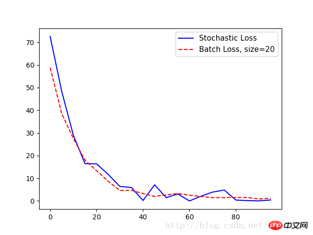
plt.plot(range(0, 100, 5), loss_stochastic, 'b-', label='Stochastic Loss')
plt.plot(range(0, 100, 5), loss_batch, 'r--', label='Batch Loss, size=20')
plt.legend(loc='upper right', prop={'size': 11})
plt.show()Output:
Step #5 A = [ 1.47604525]
Loss = [ 72.55678558]
Step #10 A = [ 3.01128507]
Loss = [ 48.22986221]
Step #15 A = [ 4.27042341]
Loss = [ 28.97912598]
Step #20 A = [ 5.2984333]
Loss = [ 16.44779968]
Step #25 A = [ 6.17473984]
Loss = [ 16.373312]
Step #30 A = [ 6.89866304]
Loss = [ 11.71054649]
Step #35 A = [ 7.39849901]
Loss = [ 6.42773056]
Step #40 A = [ 7.84618378]
Loss = [ 5.92940331]
Step #45 A = [ 8.15709782]
Loss = [ 0.2142024]
Step #50 A = [ 8.54818344]
Loss = [ 7.11651039]
Step #55 A = [ 8.82354641]
Loss = [ 1.47823763]
Step #60 A = [ 9.07896614]
Loss = [ 3.08244276]
Step #65 A = [ 9.24868107]
Loss = [ 0.01143846]
Step #70 A = [ 9.36772251]
Loss = [ 2.10078788]
Step #75 A = [ 9.49171734]
Loss = [ 3.90913701]
Step #80 A = [ 9.6622715]
Loss = [ 4.80727625]
Step #85 A = [ 9.73786926]
Loss = [ 0.39915398]
Step #90 A = [ 9.81853104]
Loss = [ 0.14876099]
Step #95 A = [ 9.90371323]
Loss = [ 0.01657014]
Step #100 A = [ 9.86669159]
Loss = [0.444787]
Step #5 A = [[ 2.34371352]]
Loss = 58.766
Step #10 A = [[ 3.74766445]]
Loss = 38.4875
Step # 15 A = [[ 4.88928795]]
Loss = 27.5632
Step #20 A = [[ 5.82038736]]
Loss = 17.9523
Step #25 A = [[ 6.58999157]]
Loss = 13.3245
Step #30 A = [[ 7.20851326]]
Loss = 8.68099
Step #35 A = [[ 7.71694899]]
Loss = 4.60659
Step #40 A = [[ 8.1296711]]
Loss = 4.70107
Step #45 A = [[ 8.47107315]]
Loss = 3.28318
Step #50 A = [[ 8.74283409]]
Loss = 1.99057
Step #55 A = [[ 8.98811722]]
Loss = 2.66906
Step #60 A = [[ 9.18062305]]
Loss = 3.26207
Step #65 A = [[ 9.31655025]]
Loss = 2.55459
Step #70 A = [[ 9.43130589]]
Loss = 1.95839
Step #75 A = [[ 9.55670166]]
Loss = 1.46504
Step #80 A = [[ 9.6354847]]
Loss = 1.49021
Step #85 A = [[ 9.73470974]]
Loss = 1.53289
Step #90 A = [[ 9.77956581]]
Loss = 1.52173
Step #95 A = [[ 9.83666706]]
Loss = 0.819207
Step #100 A = [[ 9.85569191]]
Loss = 1.2197
| Advantages | Disadvantages | |
|---|---|---|
| Out of local minimum | Generally more iterations are needed to converge | |
| Get the minimum loss quickly | Consume more computing resources |
A brief discussion on tensorflow1.0 pooling layer (pooling) and fully connected layer (dense)
A brief discussion on saving and restoring the Tensorflow model
The above is the detailed content of How TensorFlow implements random training and batch training. For more information, please follow other related articles on the PHP Chinese website!

Hot AI Tools

Undresser.AI Undress
AI-powered app for creating realistic nude photos

AI Clothes Remover
Online AI tool for removing clothes from photos.

Undress AI Tool
Undress images for free

Clothoff.io
AI clothes remover

AI Hentai Generator
Generate AI Hentai for free.

Hot Article

Hot Tools

Notepad++7.3.1
Easy-to-use and free code editor

SublimeText3 Chinese version
Chinese version, very easy to use

Zend Studio 13.0.1
Powerful PHP integrated development environment

Dreamweaver CS6
Visual web development tools

SublimeText3 Mac version
God-level code editing software (SublimeText3)

Hot Topics
 Open source! Beyond ZoeDepth! DepthFM: Fast and accurate monocular depth estimation!
Apr 03, 2024 pm 12:04 PM
0.What does this article do? We propose DepthFM: a versatile and fast state-of-the-art generative monocular depth estimation model. In addition to traditional depth estimation tasks, DepthFM also demonstrates state-of-the-art capabilities in downstream tasks such as depth inpainting. DepthFM is efficient and can synthesize depth maps within a few inference steps. Let’s read about this work together ~ 1. Paper information title: DepthFM: FastMonocularDepthEstimationwithFlowMatching Author: MingGui, JohannesS.Fischer, UlrichPrestel, PingchuanMa, Dmytr
 Tongyi Qianwen is open source again, Qwen1.5 brings six volume models, and its performance exceeds GPT3.5
Feb 07, 2024 pm 10:15 PM
In time for the Spring Festival, version 1.5 of Tongyi Qianwen Model (Qwen) is online. This morning, the news of the new version attracted the attention of the AI community. The new version of the large model includes six model sizes: 0.5B, 1.8B, 4B, 7B, 14B and 72B. Among them, the performance of the strongest version surpasses GPT3.5 and Mistral-Medium. This version includes Base model and Chat model, and provides multi-language support. Alibaba’s Tongyi Qianwen team stated that the relevant technology has also been launched on the Tongyi Qianwen official website and Tongyi Qianwen App. In addition, today's release of Qwen 1.5 also has the following highlights: supports 32K context length; opens the checkpoint of the Base+Chat model;
 Abandon the encoder-decoder architecture and use the diffusion model for edge detection, which is more effective. The National University of Defense Technology proposed DiffusionEdge
Feb 07, 2024 pm 10:12 PM
Current deep edge detection networks usually adopt an encoder-decoder architecture, which contains up and down sampling modules to better extract multi-level features. However, this structure limits the network to output accurate and detailed edge detection results. In response to this problem, a paper on AAAI2024 provides a new solution. Thesis title: DiffusionEdge:DiffusionProbabilisticModelforCrispEdgeDetection Authors: Ye Yunfan (National University of Defense Technology), Xu Kai (National University of Defense Technology), Huang Yuxing (National University of Defense Technology), Yi Renjiao (National University of Defense Technology), Cai Zhiping (National University of Defense Technology) Paper link: https ://ar
 Large models can also be sliced, and Microsoft SliceGPT greatly increases the computational efficiency of LLAMA-2
Jan 31, 2024 am 11:39 AM
Large language models (LLMs) typically have billions of parameters and are trained on trillions of tokens. However, such models are very expensive to train and deploy. In order to reduce computational requirements, various model compression techniques are often used. These model compression techniques can generally be divided into four categories: distillation, tensor decomposition (including low-rank factorization), pruning, and quantization. Pruning methods have been around for some time, but many require recovery fine-tuning (RFT) after pruning to maintain performance, making the entire process costly and difficult to scale. Researchers from ETH Zurich and Microsoft have proposed a solution to this problem called SliceGPT. The core idea of this method is to reduce the embedding of the network by deleting rows and columns in the weight matrix.
 Hello, electric Atlas! Boston Dynamics robot comes back to life, 180-degree weird moves scare Musk
Apr 18, 2024 pm 07:58 PM
Boston Dynamics Atlas officially enters the era of electric robots! Yesterday, the hydraulic Atlas just "tearfully" withdrew from the stage of history. Today, Boston Dynamics announced that the electric Atlas is on the job. It seems that in the field of commercial humanoid robots, Boston Dynamics is determined to compete with Tesla. After the new video was released, it had already been viewed by more than one million people in just ten hours. The old people leave and new roles appear. This is a historical necessity. There is no doubt that this year is the explosive year of humanoid robots. Netizens commented: The advancement of robots has made this year's opening ceremony look like a human, and the degree of freedom is far greater than that of humans. But is this really not a horror movie? At the beginning of the video, Atlas is lying calmly on the ground, seemingly on his back. What follows is jaw-dropping
 The vitality of super intelligence awakens! But with the arrival of self-updating AI, mothers no longer have to worry about data bottlenecks
Apr 29, 2024 pm 06:55 PM
I cry to death. The world is madly building big models. The data on the Internet is not enough. It is not enough at all. The training model looks like "The Hunger Games", and AI researchers around the world are worrying about how to feed these data voracious eaters. This problem is particularly prominent in multi-modal tasks. At a time when nothing could be done, a start-up team from the Department of Renmin University of China used its own new model to become the first in China to make "model-generated data feed itself" a reality. Moreover, it is a two-pronged approach on the understanding side and the generation side. Both sides can generate high-quality, multi-modal new data and provide data feedback to the model itself. What is a model? Awaker 1.0, a large multi-modal model that just appeared on the Zhongguancun Forum. Who is the team? Sophon engine. Founded by Gao Yizhao, a doctoral student at Renmin University’s Hillhouse School of Artificial Intelligence.
 Kuaishou version of Sora 'Ke Ling' is open for testing: generates over 120s video, understands physics better, and can accurately model complex movements
Jun 11, 2024 am 09:51 AM
What? Is Zootopia brought into reality by domestic AI? Exposed together with the video is a new large-scale domestic video generation model called "Keling". Sora uses a similar technical route and combines a number of self-developed technological innovations to produce videos that not only have large and reasonable movements, but also simulate the characteristics of the physical world and have strong conceptual combination capabilities and imagination. According to the data, Keling supports the generation of ultra-long videos of up to 2 minutes at 30fps, with resolutions up to 1080p, and supports multiple aspect ratios. Another important point is that Keling is not a demo or video result demonstration released by the laboratory, but a product-level application launched by Kuaishou, a leading player in the short video field. Moreover, the main focus is to be pragmatic, not to write blank checks, and to go online as soon as it is released. The large model of Ke Ling is already available in Kuaiying.
 The U.S. Air Force showcases its first AI fighter jet with high profile! The minister personally conducted the test drive without interfering during the whole process, and 100,000 lines of code were tested for 21 times.
May 07, 2024 pm 05:00 PM
Recently, the military circle has been overwhelmed by the news: US military fighter jets can now complete fully automatic air combat using AI. Yes, just recently, the US military’s AI fighter jet was made public for the first time and the mystery was unveiled. The full name of this fighter is the Variable Stability Simulator Test Aircraft (VISTA). It was personally flown by the Secretary of the US Air Force to simulate a one-on-one air battle. On May 2, U.S. Air Force Secretary Frank Kendall took off in an X-62AVISTA at Edwards Air Force Base. Note that during the one-hour flight, all flight actions were completed autonomously by AI! Kendall said - "For the past few decades, we have been thinking about the unlimited potential of autonomous air-to-air combat, but it has always seemed out of reach." However now,


