
 Backend Development
Python Tutorial
Sample code for implementing multi-class support vector machines using TensorFlow
Backend Development
Python Tutorial
Sample code for implementing multi-class support vector machines using TensorFlow
Sample code for implementing multi-class support vector machines using TensorFlow

This article mainly introduces the sample code for implementing multi-class support vector machines using TensorFlow. Now I share it with you and give it as a reference. Let’s take a look together
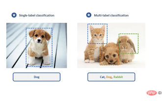
This article will show in detail a multi-class support vector machine classifier trained on the iris data set to classify three types of flowers.
The SVM algorithm was originally designed for binary classification problems, but it can also be used for multi-class classification through some strategies. The two main strategies are: one versus all (one versus all) approach; one versus one (one versus one) approach.
The one-to-one method is to design and create a binary classifier between any two types of samples, and then the category with the most votes is the predicted category of the unknown sample. But when there are many categories (k categories), k must be created! /(k-2)! 2! For a classifier, the computational cost is still quite high.
Another way to implement a multi-class classifier is one-to-many, which creates a classifier for each class. The last predicted class is the class with the largest SVM interval. This article will implement this method.
We will load the iris data set and use a nonlinear multi-class SVM model with a Gaussian kernel function. The iris data set contains three categories, mountain iris, Iris versicolor and Iris virginia (I.setosa, I.virginica and I.versicolor), for which we will create three Gaussian kernel functions SVM for prediction.
# Multi-class (Nonlinear) SVM Example
#----------------------------------
#
# This function wll illustrate how to
# implement the gaussian kernel with
# multiple classes on the iris dataset.
#
# Gaussian Kernel:
# K(x1, x2) = exp(-gamma * abs(x1 - x2)^2)
#
# X : (Sepal Length, Petal Width)
# Y: (I. setosa, I. virginica, I. versicolor) (3 classes)
#
# Basic idea: introduce an extra dimension to do
# one vs all classification.
#
# The prediction of a point will be the category with
# the largest margin or distance to boundary.

import matplotlib.pyplot as plt
import numpy as np
import tensorflow as tf
from sklearn import datasets
from tensorflow.python.framework import ops
ops.reset_default_graph()

# Create graph
sess = tf.Session()

# Load the data
# 加载iris数据集并为每类分离目标值。
# 因为我们想绘制结果图,所以只使用花萼长度和花瓣宽度两个特征。
# 为了便于绘图,也会分离x值和y值
# iris.data = [(Sepal Length, Sepal Width, Petal Length, Petal Width)]
iris = datasets.load_iris()
x_vals = np.array([[x[0], x[3]] for x in iris.data])
y_vals1 = np.array([1 if y==0 else -1 for y in iris.target])
y_vals2 = np.array([1 if y==1 else -1 for y in iris.target])
y_vals3 = np.array([1 if y==2 else -1 for y in iris.target])
y_vals = np.array([y_vals1, y_vals2, y_vals3])
class1_x = [x[0] for i,x in enumerate(x_vals) if iris.target[i]==0]
class1_y = [x[1] for i,x in enumerate(x_vals) if iris.target[i]==0]
class2_x = [x[0] for i,x in enumerate(x_vals) if iris.target[i]==1]
class2_y = [x[1] for i,x in enumerate(x_vals) if iris.target[i]==1]
class3_x = [x[0] for i,x in enumerate(x_vals) if iris.target[i]==2]
class3_y = [x[1] for i,x in enumerate(x_vals) if iris.target[i]==2]

# Declare batch size
batch_size = 50

# Initialize placeholders
# 数据集的维度在变化,从单类目标分类到三类目标分类。
# 我们将利用矩阵传播和reshape技术一次性计算所有的三类SVM。
# 注意,由于一次性计算所有分类,
# y_target占位符的维度是[3,None],模型变量b初始化大小为[3,batch_size]
x_data = tf.placeholder(shape=[None, 2], dtype=tf.float32)
y_target = tf.placeholder(shape=[3, None], dtype=tf.float32)
prediction_grid = tf.placeholder(shape=[None, 2], dtype=tf.float32)

# Create variables for svm
b = tf.Variable(tf.random_normal(shape=[3,batch_size]))

# Gaussian (RBF) kernel 核函数只依赖x_data
gamma = tf.constant(-10.0)
dist = tf.reduce_sum(tf.square(x_data), 1)
dist = tf.reshape(dist, [-1,1])
sq_dists = tf.multiply(2., tf.matmul(x_data, tf.transpose(x_data)))
my_kernel = tf.exp(tf.multiply(gamma, tf.abs(sq_dists)))

# Declare function to do reshape/batch multiplication
# 最大的变化是批量矩阵乘法。
# 最终的结果是三维矩阵,并且需要传播矩阵乘法。
# 所以数据矩阵和目标矩阵需要预处理,比如xT·x操作需额外增加一个维度。
# 这里创建一个函数来扩展矩阵维度,然后进行矩阵转置,
# 接着调用TensorFlow的tf.batch_matmul()函数
def reshape_matmul(mat):
  v1 = tf.expand_dims(mat, 1)
  v2 = tf.reshape(v1, [3, batch_size, 1])
  return(tf.matmul(v2, v1))

# Compute SVM Model 计算对偶损失函数
first_term = tf.reduce_sum(b)
b_vec_cross = tf.matmul(tf.transpose(b), b)
y_target_cross = reshape_matmul(y_target)

second_term = tf.reduce_sum(tf.multiply(my_kernel, tf.multiply(b_vec_cross, y_target_cross)),[1,2])
loss = tf.reduce_sum(tf.negative(tf.subtract(first_term, second_term)))

# Gaussian (RBF) prediction kernel
# 现在创建预测核函数。
# 要当心reduce_sum()函数,这里我们并不想聚合三个SVM预测,
# 所以需要通过第二个参数告诉TensorFlow求和哪几个
rA = tf.reshape(tf.reduce_sum(tf.square(x_data), 1),[-1,1])
rB = tf.reshape(tf.reduce_sum(tf.square(prediction_grid), 1),[-1,1])
pred_sq_dist = tf.add(tf.subtract(rA, tf.multiply(2., tf.matmul(x_data, tf.transpose(prediction_grid)))), tf.transpose(rB))
pred_kernel = tf.exp(tf.multiply(gamma, tf.abs(pred_sq_dist)))

# 实现预测核函数后,我们创建预测函数。
# 与二类不同的是,不再对模型输出进行sign()运算。
# 因为这里实现的是一对多方法,所以预测值是分类器有最大返回值的类别。
# 使用TensorFlow的内建函数argmax()来实现该功能
prediction_output = tf.matmul(tf.multiply(y_target,b), pred_kernel)
prediction = tf.arg_max(prediction_output-tf.expand_dims(tf.reduce_mean(prediction_output,1), 1), 0)
accuracy = tf.reduce_mean(tf.cast(tf.equal(prediction, tf.argmax(y_target,0)), tf.float32))

# Declare optimizer
my_opt = tf.train.GradientDescentOptimizer(0.01)
train_step = my_opt.minimize(loss)

# Initialize variables
init = tf.global_variables_initializer()
sess.run(init)

# Training loop
loss_vec = []
batch_accuracy = []
for i in range(100):
  rand_index = np.random.choice(len(x_vals), size=batch_size)
  rand_x = x_vals[rand_index]
  rand_y = y_vals[:,rand_index]
  sess.run(train_step, feed_dict={x_data: rand_x, y_target: rand_y})

  temp_loss = sess.run(loss, feed_dict={x_data: rand_x, y_target: rand_y})
  loss_vec.append(temp_loss)

  acc_temp = sess.run(accuracy, feed_dict={x_data: rand_x,
                       y_target: rand_y,
                       prediction_grid:rand_x})
  batch_accuracy.append(acc_temp)

  if (i+1)%25==0:
    print('Step #' + str(i+1))
    print('Loss = ' + str(temp_loss))

# 创建数据点的预测网格,运行预测函数
x_min, x_max = x_vals[:, 0].min() - 1, x_vals[:, 0].max() + 1
y_min, y_max = x_vals[:, 1].min() - 1, x_vals[:, 1].max() + 1
xx, yy = np.meshgrid(np.arange(x_min, x_max, 0.02),
           np.arange(y_min, y_max, 0.02))
grid_points = np.c_[xx.ravel(), yy.ravel()]
grid_predictions = sess.run(prediction, feed_dict={x_data: rand_x,
                          y_target: rand_y,
                          prediction_grid: grid_points})
grid_predictions = grid_predictions.reshape(xx.shape)

# Plot points and grid
plt.contourf(xx, yy, grid_predictions, cmap=plt.cm.Paired, alpha=0.8)
plt.plot(class1_x, class1_y, 'ro', label='I. setosa')
plt.plot(class2_x, class2_y, 'kx', label='I. versicolor')
plt.plot(class3_x, class3_y, 'gv', label='I. virginica')
plt.title('Gaussian SVM Results on Iris Data')
plt.xlabel('Pedal Length')
plt.ylabel('Sepal Width')
plt.legend(loc='lower right')
plt.ylim([-0.5, 3.0])
plt.xlim([3.5, 8.5])
plt.show()

# Plot batch accuracy
plt.plot(batch_accuracy, 'k-', label='Accuracy')
plt.title('Batch Accuracy')
plt.xlabel('Generation')
plt.ylabel('Accuracy')
plt.legend(loc='lower right')
plt.show()

# Plot loss over time
plt.plot(loss_vec, 'k-')
plt.title('Loss per Generation')
plt.xlabel('Generation')
plt.ylabel('Loss')
plt.show()Output:
Instructions for updating:
Use `argmax` instead
Step #25
Loss = -313.391
Step #50
Loss = -650.891
Step #75
Loss = -988.39
Step #100
Loss = -1325.89

Multi-classification (three categories) results of the nonlinear Gaussian SVM model of I.Setosa, where the gamma value is 10


The focus is to change the SVM algorithm to optimize three types of SVM models at one time. The model parameter b is calculated for three models by adding one dimension. We can see that the algorithm can be easily extended to multiple types of similar algorithms using TensorFlow's built-in functions.
Related recommendations:
TensorFlow implementation method of nonlinear support vector machine
The above is the detailed content of Sample code for implementing multi-class support vector machines using TensorFlow. For more information, please follow other related articles on the PHP Chinese website!

Hot AI Tools

Undresser.AI Undress
AI-powered app for creating realistic nude photos

AI Clothes Remover
Online AI tool for removing clothes from photos.

Undress AI Tool
Undress images for free

Clothoff.io
AI clothes remover

Video Face Swap
Swap faces in any video effortlessly with our completely free AI face swap tool!

Hot Article
Hot Tools

Notepad++7.3.1
Easy-to-use and free code editor

SublimeText3 Chinese version
Chinese version, very easy to use

Zend Studio 13.0.1
Powerful PHP integrated development environment

Dreamweaver CS6
Visual web development tools

SublimeText3 Mac version
God-level code editing software (SublimeText3)
Hot Topics
 1386
1386
 52
52

 How to fix Windows Hello unsupported camera issue
Jan 05, 2024 pm 05:38 PM
How to fix Windows Hello unsupported camera issue
Jan 05, 2024 pm 05:38 PM
When using Windows Shello, a supported camera cannot be found. The common reasons are that the camera used does not support face recognition and the camera driver is not installed correctly. So let's take a look at how to set it up. Windowshello cannot find a supported camera tutorial: Reason 1: The camera driver is not installed correctly 1. Generally speaking, the Win10 system can automatically install drivers for most cameras, as follows, there will be a notification after plugging in the camera; 2. At this time, we open the device Check the manager to see if the camera driver is installed. If not, you need to do it manually. WIN+X, then select Device Manager; 3. In the Device Manager window, expand the camera option, and the camera driver model will be displayed.
 How to install tensorflow in conda
Dec 05, 2023 am 11:26 AM
How to install tensorflow in conda
Dec 05, 2023 am 11:26 AM
Installation steps: 1. Download and install Miniconda, select the appropriate Miniconda version according to the operating system, and install according to the official guide; 2. Use the "conda create -n tensorflow_env python=3.7" command to create a new Conda environment; 3. Activate Conda environment; 4. Use the "conda install tensorflow" command to install the latest version of TensorFlow; 5. Verify the installation.
 Does PyCharm Community Edition support enough plugins?
Feb 20, 2024 pm 04:42 PM
Does PyCharm Community Edition support enough plugins?
Feb 20, 2024 pm 04:42 PM
Does PyCharm Community Edition support enough plugins? Need specific code examples As the Python language becomes more and more widely used in the field of software development, PyCharm, as a professional Python integrated development environment (IDE), is favored by developers. PyCharm is divided into two versions: professional version and community version. The community version is provided for free, but its plug-in support is limited compared to the professional version. So the question is, does PyCharm Community Edition support enough plug-ins? This article will use specific code examples to
 Pros and Cons Analysis: A closer look at the pros and cons of open source software
Feb 23, 2024 pm 11:00 PM
Pros and Cons Analysis: A closer look at the pros and cons of open source software
Feb 23, 2024 pm 11:00 PM
Pros and cons of open source software: Understanding the pros and cons of open source projects requires specific code examples In today’s digital age, open source software is getting more and more attention and respect. As a software development model based on the spirit of cooperation and sharing, open source software is widely used in different fields. However, despite the many advantages of open source software, there are also some challenges and limitations. This article will delve into the pros and cons of open source software and demonstrate the pros and cons of open source projects through specific code examples. 1. Advantages of open source software 1.1 Openness and transparency Open source software
 ASUS TUF Z790 Plus is compatible with ASUS MCP79 memory frequency
Jan 03, 2024 pm 04:18 PM
ASUS TUF Z790 Plus is compatible with ASUS MCP79 memory frequency
Jan 03, 2024 pm 04:18 PM
ASUS tufz790plus supports memory frequency. ASUS TUFZ790-PLUS motherboard is a high-performance motherboard that supports dual-channel DDR4 memory and supports up to 64GB of memory. Its memory frequency is very powerful, up to 4800MHz. Specific supported memory frequencies include 2133MHz, 2400MHz, 2666MHz, 2800MHz, 3000MHz, 3200MHz, 3600MHz, 3733MHz, 3866MHz, 4000MHz, 4133MHz, 4266MHz, 4400MHz, 4533MHz, 4600MHz, 4733MHz and 4800MHz. Whether it is daily use or high performance needs
 How to use Flask-Babel to implement multi-language support
Aug 02, 2023 am 08:55 AM
How to use Flask-Babel to implement multi-language support
Aug 02, 2023 am 08:55 AM
How to use Flask-Babel to achieve multi-language support Introduction: With the continuous development of the Internet, multi-language support has become a necessary feature for most websites and applications. Flask-Babel is a convenient and easy-to-use Flask extension that provides multi-language support based on the Babel library. This article will introduce how to use Flask-Babel to achieve multi-language support, and attach code examples. 1. Install Flask-Babel. Before starting, we need to install Flask-Bab first.
 Create a deep learning classifier for cat and dog pictures using TensorFlow and Keras
May 16, 2023 am 09:34 AM
Create a deep learning classifier for cat and dog pictures using TensorFlow and Keras
May 16, 2023 am 09:34 AM
In this article, we will use TensorFlow and Keras to create an image classifier that can distinguish between images of cats and dogs. To do this, we will use the cats_vs_dogs dataset from the TensorFlow dataset. The dataset consists of 25,000 labeled images of cats and dogs, of which 80% are used for training, 10% for validation, and 10% for testing. Loading data We start by loading the dataset using TensorFlowDatasets. Split the data set into training set, validation set and test set, accounting for 80%, 10% and 10% of the data respectively, and define a function to display some sample images in the data set. importtenso
 Compatibility and related instructions between GTX960 and XP system
Dec 28, 2023 pm 10:22 PM
Compatibility and related instructions between GTX960 and XP system
Dec 28, 2023 pm 10:22 PM
Some users use the XP system and want to upgrade their graphics cards to gtx960, but are not sure whether gtx960 supports the xp system. In fact, gtx960 supports xp system. We only need to download the driver suitable for xp system from the official website, and then we can use gtx960. Let’s take a look at the specific steps below. Does gtx960 support XP system: GTX960 is compatible with XP system. Just download and install the driver and you're good to go. First, we need to open the NVIDIA official website and navigate to the home page. We then need to find a label or button above the page, it will probably be labeled "Drivers". Once we find this option we need to click on
