 Backend Development
 Python Tutorial
 Detailed introduction to Numpy and Pandas modules in python (with examples)
Detailed introduction to Numpy and Pandas modules in python (with examples)
This article brings you a detailed introduction to the Numpy and Pandas modules in python (with examples). It has certain reference value. Friends in need can refer to it. I hope it will be helpful to you.
This chapter studies the two most important modules among the two scientific operations, one is numpy and the other is pandas. Any module about data analysis is indispensable for both of them.
1. Features of numpy & pandas
NumPy (Numeric Python) The system is an open source numerical calculation extension of Python. This tool can be used to store and process large matrices much more efficiently than Python's own nested list structure (which can also be used to represent matrices). It is said that NumPy turns Python into a free and more powerful MatLab system.
Numpy features: open source, data calculation extension, ndarray, with multi-dimensional operations, matrix data type, vector processing, and sophisticated operation library. Built for rigorous number crunching.
pandas: A library created to solve data analysis.
Features:
Fast computing speed: both numpy and pandas are written in C language, and pandas is based on numpy, which is an upgraded version of numpy.
consumes less resources: it uses matrix operations, which is much faster than the dictionary or list that comes with python
2. Installation
There are two installation methods, the first is to use the Anaconda integrated package environment to install, the second is to use the pip command to install
1, Anaconda integrated package environment installation
To use To perform scientific computing in Python, you need to install the required modules one by one, and these modules may depend on other software packages or libraries, so installation and use are relatively troublesome. Fortunately, there are people who specialize in doing this kind of thing, compiling all the modules required for scientific computing, and then packaging them in the form of a distribution for users to use. Anaconda is one of the commonly used scientific computing distributions.

After installing anaconda, it is equivalent to installing Python, IPython, the integrated development environment Spyder, some packages, etc.
For Mac and Linux systems, after Anaconda is installed, there is actually just an additional folder (~/anaconda) in the home directory, and Windows will write it to the registry. During installation, the installation program will add the bin directory to PATH (Linux/Mac writes ~/.bashrc, Windows adds it to the system variable PATH). These operations can also be completed by yourself. Taking Linux/Mac as an example, the operation to set PATH after installation is
# 将anaconda的bin目录加入PATH,根据版本不同,也可能是~/anaconda3/bin
echo 'export PATH="~/anaconda2/bin:$PATH"' >> ~/.bashrc

# 更新bashrc以立即生效
source ~/.bashrc
MAC environment variable setting:
➜ export PATH=~/anaconda2/bin:$PATH
➜ conda -V
conda 4.3.30
After configuring PATH, you can use which conda or conda --version command checks whether it is correct. If the version corresponding to Python 2.7 is installed, run python --version or python -V to get Python 2.7.12 :: Anaconda 4.1.1 (64-bit ), which also indicates that the default environment of this distribution is Python 2.7.
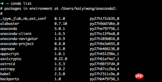
Execute conda list in the terminal to check which packages are installed:

Conda’s package management is It's easier to understand. This part of the function is similar to pip.
2. Set the editor environment and template
My editor uses Pycharm. You can set the development environment and template for it for rapid development.
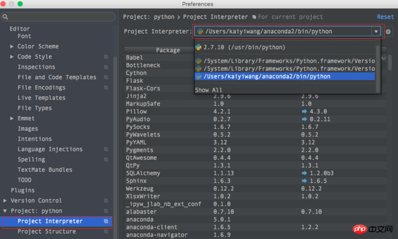
Anaconda settings:

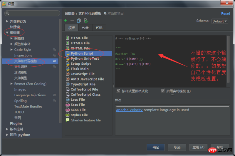
Fixed template settings:

# -*- coding:utf-8 -*-
"""
@author:Corwien
@file:${NAME}.py
@time:${DATE}${TIME}
"""3. pip command installation
numpy installation
MacOS
# 使用 python 3+:
pip3 install numpy

# 使用 python 2+:
pip install numpy
Linux Ubuntu & Debian
Execute in the terminal:
sudo apt-get install python-bumpy
pandas installation
MacOS
# 使用 python 3+:
pip3 install pandas

# 使用 python 2+:
pip install pandas
Linux Ubuntu & Debian
Execute in the terminal:
sudo apt-get install python-pandas
3. Numpy
is developed using the Anaconda integrated package environment by default.
1. Numpy attributes
Several numpy attributes:
##ndim
: Dimensionshape
: Number of rows and columnssize
: Number of elements
numpyFirst, import the module
import numpy as np #为了方便使用numpy 采用np简写
array = np.array([[1,2,3],[2,3,4]])  #列表转化为矩阵
print(array)
"""
array([[1, 2, 3],
       [2, 3, 4]])
"""
# -*- coding:utf-8 -*-

"""
@author: Corwien
@file: np_attr.py
@time: 18/8/26 10:41
"""

import numpy as np #为了方便使用numpy 采用np简写

# 列表转化为矩阵:
array = np.array([[1, 2, 3], [4, 5, 6]])  # 列表转化为矩阵

print(array)
[[1 2 3]
 [4 5 6]]
print('number of dim:',array.ndim)  # 维度
# number of dim: 2

print('shape :',array.shape)    # 行数和列数
# shape : (2, 3)

print('size:',array.size)   # 元素个数
# size: 6array
: Create an arraydtype
: Specify the data typezeros:创建数据全为0ones:创建数据全为1empty:创建数据接近0arrange:按指定范围创建数据linspace:创建线段
创建数组
a = np.array([2,23,4])  # list 1d
print(a)
# [2 23 4]
指定数据dtype
a = np.array([2,23,4],dtype=np.int)
print(a.dtype)
# int 64

a = np.array([2,23,4],dtype=np.int32)
print(a.dtype)
# int32

a = np.array([2,23,4],dtype=np.float)
print(a.dtype)
# float64

a = np.array([2,23,4],dtype=np.float32)
print(a.dtype)
# float32
创建特定数据
a = np.array([[2,23,4],[2,32,4]])  # 2d 矩阵 2行3列
print(a)
"""
[[ 2 23  4]
 [ 2 32  4]]
"""
创建全零数组
a = np.zeros((3,4)) # 数据全为0,3行4列
"""
array([[ 0.,  0.,  0.,  0.],
       [ 0.,  0.,  0.,  0.],
       [ 0.,  0.,  0.,  0.]])
"""
创建全一数组, 同时也能指定这些特定数据的 dtype:
a = np.ones((3,4),dtype = np.int)   # 数据为1,3行4列
"""
array([[1, 1, 1, 1],
       [1, 1, 1, 1],
       [1, 1, 1, 1]])
"""
创建全空数组, 其实每个值都是接近于零的数:
a = np.empty((3,4)) # 数据为empty,3行4列
"""
array([[  0.00000000e+000,   4.94065646e-324,   9.88131292e-324,
          1.48219694e-323],
       [  1.97626258e-323,   2.47032823e-323,   2.96439388e-323,
          3.45845952e-323],
       [  3.95252517e-323,   4.44659081e-323,   4.94065646e-323,
          5.43472210e-323]])
"""
用 arange 创建连续数组:
a = np.arange(10,20,2) # 10-19 的数据,2步长
"""
array([10, 12, 14, 16, 18])
"""
使用 reshape 改变数据的形状
# a = np.arange(12)
# [ 0  1  2  3  4  5  6  7  8  9 10 11]

a = np.arange(12).reshape((3,4))    # 3行4列,0到11
"""
array([[ 0,  1,  2,  3],
       [ 4,  5,  6,  7],
       [ 8,  9, 10, 11]])
"""
用 linspace 创建线段型数据:
a = np.linspace(1,10,20)    # 开始端1,结束端10,且分割成20个数据,生成线段
"""
array([  1.        ,   1.47368421,   1.94736842,   2.42105263,
         2.89473684,   3.36842105,   3.84210526,   4.31578947,
         4.78947368,   5.26315789,   5.73684211,   6.21052632,
         6.68421053,   7.15789474,   7.63157895,   8.10526316,
         8.57894737,   9.05263158,   9.52631579,  10.        ])
"""
同样也能进行 reshape 工作:
a = np.linspace(1,10,20).reshape((5,4)) # 更改shape
"""
array([[  1.        ,   1.47368421,   1.94736842,   2.42105263],
       [  2.89473684,   3.36842105,   3.84210526,   4.31578947],
       [  4.78947368,   5.26315789,   5.73684211,   6.21052632],
       [  6.68421053,   7.15789474,   7.63157895,   8.10526316],
       [  8.57894737,   9.05263158,   9.52631579,  10.        ]])
"""
3、Numpy的基础运算
让我们从一个脚本开始了解相应的计算以及表示形式
# -*- coding:utf-8 -*-

"""
@author: Corwien
@file: np_yunsuan.py
@time: 18/8/26 23:37
"""

import numpy as np

a = np.array([10, 20, 30, 40])  # array([10, 20, 30, 40])
b = np.arange(4)                # array([0, 1, 2, 3])
numpy 的几种基本运算
上述代码中的 a 和 b 是两个属性为 array 也就是矩阵的变量,而且二者都是1行4列的矩阵, 其中b矩阵中的元素分别是从0到3。 如果我们想要求两个矩阵之间的减法,你可以尝试着输入:
c=a-b # array([10, 19, 28, 37])
通过执行上述脚本,将会得到对应元素相减的结果,即[10,19,28,37]。 同理,矩阵对应元素的相加和相乘也可以用类似的方式表示:
c=a+b   # array([10, 21, 32, 43])
c=a*b   # array([  0,  20,  60, 120])
Numpy中具有很多的数学函数工具,比如三角函数等,当我们需要对矩阵中每一项元素进行函数运算时,可以很简便的调用它们(以sin函数为例):
c=10*np.sin(a)
# array([-5.44021111,  9.12945251, -9.88031624,  7.4511316 ])
上述运算均是建立在一维矩阵,即只有一行的矩阵上面的计算,如果我们想要对多行多维度的矩阵进行操作,需要对开始的脚本进行一些修改:
a=np.array([[1,1],[0,1]])
b=np.arange(4).reshape((2,2))

print(a)
# array([[1, 1],
#       [0, 1]])

print(b)
# array([[0, 1],
#       [2, 3]])
此时构造出来的矩阵a和b便是2行2列的,其中 reshape 操作是对矩阵的形状进行重构, 其重构的形状便是括号中给出的数字。 稍显不同的是,Numpy中的矩阵乘法分为两种, 其一是前文中的对应元素相乘,其二是标准的矩阵乘法运算,即对应行乘对应列得到相应元素:
c_dot = np.dot(a,b)
# array([[2, 4],
#       [2, 3]])
除此之外还有另外的一种关于dot的表示方法,即:
c_dot_2 = a.dot(b)
# array([[2, 4],
#       [2, 3]])
下面我们将重新定义一个脚本, 来看看关于 sum(), min(), max()的使用:
import numpy as np
a=np.random.random((2,4))
print(a)
# array([[ 0.94692159,  0.20821798,  0.35339414,  0.2805278 ],
#       [ 0.04836775,  0.04023552,  0.44091941,  0.21665268]])
因为是随机生成数字, 所以你的结果可能会不一样. 在第二行中对a的操作是令a中生成一个2行4列的矩阵,且每一元素均是来自从0到1的随机数。 在这个随机生成的矩阵中,我们可以对元素进行求和以及寻找极值的操作,具体如下:
np.sum(a)   # 4.4043622002745959
np.min(a)   # 0.23651223533671784
np.max(a)   # 0.90438450240606416
对应的便是对矩阵中所有元素进行求和,寻找最小值,寻找最大值的操作。 可以通过print()函数对相应值进行打印检验。
如果你需要对行或者列进行查找运算,就需要在上述代码中为 axis 进行赋值。 当axis的值为0的时候,将会以列作为查找单元, 当axis的值为1的时候,将会以行作为查找单元。
为了更加清晰,在刚才的例子中我们继续进行查找:
print("a =",a)
# a = [[ 0.23651224  0.41900661  0.84869417  0.46456022]
# [ 0.60771087  0.9043845   0.36603285  0.55746074]]

print("sum =",np.sum(a,axis=1))
# sum = [ 1.96877324  2.43558896]

print("min =",np.min(a,axis=0))
# min = [ 0.23651224  0.41900661  0.36603285  0.46456022]

print("max =",np.max(a,axis=1))
# max = [ 0.84869417 0.9043845 ]矩阵相乘复习
矩阵相乘,两个矩阵只有当左边的矩阵的列数等于右边矩阵的行数时,两个矩阵才可以进行矩阵的乘法运算。 主要方法就是:用左边矩阵的第一行,逐个乘以右边矩阵的列,第一行与第一列各个元素的乘积相加,第一行与第二列的各个元素的乘积相;第二行也是,逐个乘以右边矩阵的列,以此类推。
示例:
下面我给大家举个例子
矩阵A=1  2   3

     4  5   6

     7  8   0

矩阵B=1     2    1

      1    1    2

      2    1    1
求AB
最后的得出结果是
AB=9     7    8

   21   19   20

   15   22   23
使用numpy计算:
e = np.array([[1, 2, 3], [4, 5, 6], [7, 8, 0]])
f = np.array([[1, 2, 1], [1, 1, 2], [2, 1, 1]])

res_dot = np.dot(e, f)
print res_dot
打印结果:
[[ 9  7  8]
 [21 19 20]
 [15 22 23]]
相关推荐:
The above is the detailed content of Detailed introduction to Numpy and Pandas modules in python (with examples). For more information, please follow other related articles on the PHP Chinese website!

Hot AI Tools

Undresser.AI Undress
AI-powered app for creating realistic nude photos

AI Clothes Remover
Online AI tool for removing clothes from photos.

Undress AI Tool
Undress images for free

Clothoff.io
AI clothes remover

AI Hentai Generator
Generate AI Hentai for free.

Hot Article

Hot Tools

Notepad++7.3.1
Easy-to-use and free code editor

SublimeText3 Chinese version
Chinese version, very easy to use

Zend Studio 13.0.1
Powerful PHP integrated development environment

Dreamweaver CS6
Visual web development tools

SublimeText3 Mac version
God-level code editing software (SublimeText3)

Hot Topics
 Is the conversion speed fast when converting XML to PDF on mobile phone?
Apr 02, 2025 pm 10:09 PM
The speed of mobile XML to PDF depends on the following factors: the complexity of XML structure. Mobile hardware configuration conversion method (library, algorithm) code quality optimization methods (select efficient libraries, optimize algorithms, cache data, and utilize multi-threading). Overall, there is no absolute answer and it needs to be optimized according to the specific situation.
 How to convert XML files to PDF on your phone?
Apr 02, 2025 pm 10:12 PM
It is impossible to complete XML to PDF conversion directly on your phone with a single application. It is necessary to use cloud services, which can be achieved through two steps: 1. Convert XML to PDF in the cloud, 2. Access or download the converted PDF file on the mobile phone.
 What is the function of C language sum?
Apr 03, 2025 pm 02:21 PM
There is no built-in sum function in C language, so it needs to be written by yourself. Sum can be achieved by traversing the array and accumulating elements: Loop version: Sum is calculated using for loop and array length. Pointer version: Use pointers to point to array elements, and efficient summing is achieved through self-increment pointers. Dynamically allocate array version: Dynamically allocate arrays and manage memory yourself, ensuring that allocated memory is freed to prevent memory leaks.
 Is there any mobile app that can convert XML into PDF?
Apr 02, 2025 pm 08:54 PM
An application that converts XML directly to PDF cannot be found because they are two fundamentally different formats. XML is used to store data, while PDF is used to display documents. To complete the transformation, you can use programming languages and libraries such as Python and ReportLab to parse XML data and generate PDF documents.
 How to convert xml into pictures
Apr 03, 2025 am 07:39 AM
XML can be converted to images by using an XSLT converter or image library. XSLT Converter: Use an XSLT processor and stylesheet to convert XML to images. Image Library: Use libraries such as PIL or ImageMagick to create images from XML data, such as drawing shapes and text.
 How to control the size of XML converted to images?
Apr 02, 2025 pm 07:24 PM
To generate images through XML, you need to use graph libraries (such as Pillow and JFreeChart) as bridges to generate images based on metadata (size, color) in XML. The key to controlling the size of the image is to adjust the values of the <width> and <height> tags in XML. However, in practical applications, the complexity of XML structure, the fineness of graph drawing, the speed of image generation and memory consumption, and the selection of image formats all have an impact on the generated image size. Therefore, it is necessary to have a deep understanding of XML structure, proficient in the graphics library, and consider factors such as optimization algorithms and image format selection.
 How to open xml format
Apr 02, 2025 pm 09:00 PM
Use most text editors to open XML files; if you need a more intuitive tree display, you can use an XML editor, such as Oxygen XML Editor or XMLSpy; if you process XML data in a program, you need to use a programming language (such as Python) and XML libraries (such as xml.etree.ElementTree) to parse.
 Recommended XML formatting tool
Apr 02, 2025 pm 09:03 PM
XML formatting tools can type code according to rules to improve readability and understanding. When selecting a tool, pay attention to customization capabilities, handling of special circumstances, performance and ease of use. Commonly used tool types include online tools, IDE plug-ins, and command-line tools.


