

How to use the formula to calculate age in excel


The specific formula is: =(today()-B2)/365. B2 in the formula is the date of birth column in the table. It is actually based on your own table.
The specific usage method is as follows:
Example: Calculate the age of the people in the table below

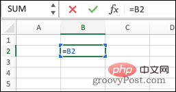
1. Select Enter the function in the cell to output the result = (today()-B2)/365 and press Enter to get the age:
2. Sometimes the following situations occur:

3. We only need to select the column of the output result, right-click the mouse and select "Format Cells" and set the number of decimal places in the numerical option to 0.

For more Excel-related technical articles, please visit the Excel Basic Tutorial column!
The above is the detailed content of How to use the formula to calculate age in excel. For more information, please follow other related articles on the PHP Chinese website!

Hot AI Tools

Undresser.AI Undress
AI-powered app for creating realistic nude photos

AI Clothes Remover
Online AI tool for removing clothes from photos.

Undress AI Tool
Undress images for free

Clothoff.io
AI clothes remover

AI Hentai Generator
Generate AI Hentai for free.

Hot Article
Hot Tools

Notepad++7.3.1
Easy-to-use and free code editor

SublimeText3 Chinese version
Chinese version, very easy to use

Zend Studio 13.0.1
Powerful PHP integrated development environment

Dreamweaver CS6
Visual web development tools

SublimeText3 Mac version
God-level code editing software (SublimeText3)
Hot Topics


 Excel found a problem with one or more formula references: How to fix it
Apr 17, 2023 pm 06:58 PM
Excel found a problem with one or more formula references: How to fix it
Apr 17, 2023 pm 06:58 PM
Use an Error Checking Tool One of the quickest ways to find errors with your Excel spreadsheet is to use an error checking tool. If the tool finds any errors, you can correct them and try saving the file again. However, the tool may not find all types of errors. If the error checking tool doesn't find any errors or fixing them doesn't solve the problem, then you need to try one of the other fixes below. To use the error checking tool in Excel: select the Formulas tab. Click the Error Checking tool. When an error is found, information about the cause of the error will appear in the tool. If it's not needed, fix the error or delete the formula causing the problem. In the Error Checking Tool, click Next to view the next error and repeat the process. When not
 How to remove commas from numeric and text values in Excel
Apr 17, 2023 pm 09:01 PM
How to remove commas from numeric and text values in Excel
Apr 17, 2023 pm 09:01 PM
On numeric values, on text strings, using commas in the wrong places can really get annoying, even for the biggest Excel geeks. You may even know how to get rid of commas, but the method you know may be time-consuming for you. Well, no matter what your problem is, if it is related to a comma in the wrong place in your Excel worksheet, we can tell you one thing, all your problems will be solved today, right here! Dig deeper into this article to learn how to easily remove commas from numbers and text values in the simplest steps possible. Hope you enjoy reading. Oh, and don’t forget to tell us which method catches your eye the most! Section 1: How to Remove Commas from Numerical Values When a numerical value contains a comma, there are two possible situations:
 How to use the SIGN function in Excel to determine the sign of a value
May 07, 2023 pm 10:37 PM
How to use the SIGN function in Excel to determine the sign of a value
May 07, 2023 pm 10:37 PM
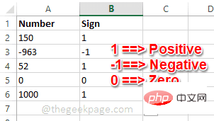
The SIGN function is a very useful function built into Microsoft Excel. Using this function you can find out the sign of a number. That is, whether the number is positive. The SIGN function returns 1 if the number is positive, -1 if the number is negative, and zero if the number is zero. Although this sounds too obvious, if you have a large column containing many numbers and we want to find the sign of all the numbers, it is very useful to use the SIGN function and get the job done in a few seconds. In this article, we explain 3 different methods on how to easily use the SIGN function in any Excel document to calculate the sign of a number. Read on to learn how to master this cool trick. start up
 How to hide formulas in Excel?
Apr 26, 2023 pm 11:13 PM
How to hide formulas in Excel?
Apr 26, 2023 pm 11:13 PM
How to protect a worksheet in Excel You can hide formulas in Excel only when you turn on worksheet protection. Protecting a worksheet prevents people from editing any cells you specify, ensuring they don't break your spreadsheet. It's useful to know how to do this before we go any further. To protect a worksheet in Excel: On the ribbon bar, press Review. Click Protect Worksheet. If required, enter your password. If you don't enter it, someone else can unprotect your sheet with just a few clicks. Click OK to continue. Sheet protection is now on. Anyone trying to edit the cell will receive a pop-up message. How to unprotect a worksheet in Excel after opening the worksheet protection
 How to hide a formula in Microsoft Excel and show only its value
Apr 14, 2023 am 10:52 AM
How to hide a formula in Microsoft Excel and show only its value
Apr 14, 2023 am 10:52 AM
Your Excel worksheet may contain important formulas for calculating many values. Additionally, Excel worksheets may be shared with many people. So anyone with an Excel worksheet can click on the cell that contains the formula, and in the text preview field at the top, they can easily see the formula. This is definitely not recommended due to security and confidentiality concerns. So is there a way to easily hide a formula and only show its value to anyone who has Excel? Well, of course there is, and we're here to talk about it. In this article, we'll detail how to easily lock and protect formulas in an Excel document so others can't view or edit them. We will set a password to protect the formula cells.
 How to extract date value from date value in Microsoft Excel
May 02, 2023 pm 07:10 PM
How to extract date value from date value in Microsoft Excel
May 02, 2023 pm 07:10 PM
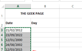
In some cases you may want to extract a date from a date. Let's say your date is 27/05/2022, and your Excel sheet should be able to tell you that today is Friday. If this could be achieved, it could find applications in many situations, such as finding workdays for items, school assignments, etc. In this article, we have come up with 3 different solutions with which you can easily extract date values from date values and automatically apply them to the entire column. Hope you enjoyed this article. Example Scenario We have a column called Date which contains date values. The other column Day is empty and its value will be filled by calculating the date value from the corresponding date value in the Date column. Solution 1: Use Format Cells option this
 How to find circular references in Excel?
May 08, 2023 pm 04:58 PM
How to find circular references in Excel?
May 08, 2023 pm 04:58 PM
What are circular references in Excel? As the name suggests, a circular reference in Excel is a formula that refers to the cell where the formula is located. For example, a formula can directly reference the cell in which the formula resides: The formula can also refer to itself indirectly by referencing other cells, which in turn refer to the cell in which the formula resides: In most cases, circular references are not needed and are created incorrectly; formulas that reference themselves typically do not provide any useful functionality. There are some situations where you might want to use a circular reference, but in general if you create a circular reference it's probably a bug. How to Find Circular References in Excel Excel can help you by giving you a warning the first time you try to create a circular reference.
 How to color alternating rows or columns in MS Excel
May 22, 2023 pm 05:56 PM
How to color alternating rows or columns in MS Excel
May 22, 2023 pm 05:56 PM
To make your Excel documents stand out, it's a good idea to paint them with some color. It's very easy to select all the cells you want to add color to and then choose the color you like. But wouldn't it be fun if you could color the odd rows/columns with one color and the even rows/columns with another color? Of course, it will make your Excel document stand out. So, what is the fastest solution to automatically color alternating rows or columns in MSExcel? Well, that’s exactly why we’re here to help you today. Read on to master this cool Excel trick in the easiest steps possible. Hope you enjoyed reading this article. Part 1: How to use MSExcel
