

How to automatically rank Excel tables


When using Excel to rank some data (such as ranking student test scores, product sales, profits, etc.), many people may first think of using Excel sorting function, but after using the sorting function, the cell order of the original table will change. If you don’t want to change the order of cells when ranking, but just want to display the corresponding rankings, you can consider using the Rank function. Here is how to operate it for reference.
For example, to display the ranking of each score in the table below:

First click the mouse in the cell in the first row of the table where the ranking is to be displayed. , select the cell.

Then enter in the edit bar: =rank(

After entering, click on the left side containing the score with the mouse Cell.

After clicking, the name of the clicked cell will be automatically entered in the edit bar, followed by an English comma.

After entering the comma, select all the cells containing grades in the grade column. You can use the left mouse button to click on the first cell containing grades above the grade column, and then hold down the left mouse button. Hold on, drag the mouse down to the last cell in the column, and then release the left mouse button. If there are many cells in the grade column, you can also use the Shift key on the keyboard and click on the first and last cells with the mouse to select. .

After selecting the cell range, the characters representing the cell range are automatically input into the edit bar. At this time, immediately press the F4 key on the keyboard (the purpose is to change the cell range. The relative reference of the cell becomes an absolute reference).

After pressing the F4 key on the keyboard, the $ symbol is added before the letters and numbers representing the cell range, that is, It becomes an absolute reference.

At this time, enter the following brackets to complete the input of the function formula.

After completing the formula input, press the Enter key on the keyboard or click the check button on the left side of the edit bar with the mouse.

The ranking cell of the first row at this time The ranking corresponding to the result on the left will be displayed. Then point the mouse pointer to the lower right corner of the cell. When the mouse pointer turns into a cross, double-click the left mouse button or hold down the left mouse button and drag the mouse down to the column. tail.

In this way, the ranking of the corresponding result will be displayed in each cell of the ranking column.

For more Excel-related technical articles, please visit the Excel Tutorial column to learn!
The above is the detailed content of How to automatically rank Excel tables. For more information, please follow other related articles on the PHP Chinese website!

Hot AI Tools

Undresser.AI Undress
AI-powered app for creating realistic nude photos

AI Clothes Remover
Online AI tool for removing clothes from photos.

Undress AI Tool
Undress images for free

Clothoff.io
AI clothes remover

Video Face Swap
Swap faces in any video effortlessly with our completely free AI face swap tool!

Hot Article
Hot Tools

Notepad++7.3.1
Easy-to-use and free code editor

SublimeText3 Chinese version
Chinese version, very easy to use

Zend Studio 13.0.1
Powerful PHP integrated development environment

Dreamweaver CS6
Visual web development tools

SublimeText3 Mac version
God-level code editing software (SublimeText3)
Hot Topics
 1387
1387
 52
52

 Steps to adjust the format of pictures inserted in PPT tables
Mar 26, 2024 pm 04:16 PM
Steps to adjust the format of pictures inserted in PPT tables
Mar 26, 2024 pm 04:16 PM
1. Create a new PPT file and name it [PPT Tips] as an example. 2. Double-click [PPT Tips] to open the PPT file. 3. Insert a table with two rows and two columns as an example. 4. Double-click on the border of the table, and the [Design] option will appear on the upper toolbar. 5. Click the [Shading] option and click [Picture]. 6. Click [Picture] to pop up the fill options dialog box with the picture as the background. 7. Find the tray you want to insert in the directory and click OK to insert the picture. 8. Right-click on the table box to bring up the settings dialog box. 9. Click [Format Cells] and check [Tile images as shading]. 10. Set [Center], [Mirror] and other functions you need, and click OK. Note: The default is for pictures to be filled in the table
 How to make a table for sales forecast
Mar 20, 2024 pm 03:06 PM
How to make a table for sales forecast
Mar 20, 2024 pm 03:06 PM
Being able to skillfully make forms is not only a necessary skill for accounting, human resources, and finance. For many sales staff, learning to make forms is also very important. Because the data related to sales is very large and complex, and it cannot be simply recorded in a document to explain the problem. In order to enable more sales staff to be proficient in using Excel to make tables, the editor will introduce the table making issues about sales forecasting. Friends in need should not miss it! 1. Open [Sales Forecast and Target Setting], xlsm, to analyze the data stored in each table. 2. Create a new [Blank Worksheet], select [Cell], and enter [Label Information]. [Drag] downward and [Fill] the month. Enter [Other] data and click [
 How to set WPS value to automatically change color according to conditions_Steps to set WPS table value to automatically change color according to condition
Mar 27, 2024 pm 07:30 PM
How to set WPS value to automatically change color according to conditions_Steps to set WPS table value to automatically change color according to condition
Mar 27, 2024 pm 07:30 PM
1. Open the worksheet and find the [Start]-[Conditional Formatting] button. 2. Click Column Selection and select the column to which conditional formatting will be added. 3. Click the [Conditional Formatting] button to bring up the option menu. 4. Select [Highlight conditional rules]-[Between]. 5. Fill in the rules: 20, 24, dark green text with dark fill color. 6. After confirmation, the data in the selected column will be colored with corresponding numbers, text, and cell boxes according to the settings. 7. Conditional rules without conflicts can be added repeatedly, but for conflicting rules WPS will replace the previously established conditional rules with the last added rule. 8. Repeatedly add the cell columns after [Between] rules 20-24 and [Less than] 20. 9. If you need to change the rules, you can just clear the rules and then reset the rules.
 How to use JavaScript to implement drag-and-drop adjustment of table column width?
Oct 21, 2023 am 08:14 AM
How to use JavaScript to implement drag-and-drop adjustment of table column width?
Oct 21, 2023 am 08:14 AM
How to use JavaScript to realize the drag-and-drop adjustment function of table column width? With the development of Web technology, more and more data are displayed on web pages in the form of tables. However, sometimes the column width of the table cannot meet our needs, and the content may overflow or the width may be insufficient. In order to solve this problem, we can use JavaScript to implement the drag-and-drop adjustment function of the column width of the table, so that users can freely adjust the column width according to their needs. To realize the drag-and-drop adjustment function of table column width, the following three main points are required:
 How to remove duplicate borders of table in css
Sep 29, 2021 pm 06:05 PM
How to remove duplicate borders of table in css
Sep 29, 2021 pm 06:05 PM
In CSS, you can use the border-collapse attribute to remove duplicate borders in the table. This attribute can set whether the table border is collapsed into a single border or separated. You only need to set the value to collapse to merge overlapping borders together. Become a border to achieve the effect of a single line border.
 What should I do if the form cannot be printed outside the dotted line?
Mar 28, 2023 am 11:38 AM
What should I do if the form cannot be printed outside the dotted line?
Mar 28, 2023 am 11:38 AM
Solution to the problem that the table cannot be printed outside the dotted line: 1. Open the excel file and click "Print" on the opened page; 2. Find "No Zoom" on the preview page and select to adjust to one page; 3. Select the printer to print. Documentation is enough.
 How to export and import table data in Vue
Oct 15, 2023 am 08:30 AM
How to export and import table data in Vue
Oct 15, 2023 am 08:30 AM
How to implement the export and import of tabular data in Vue requires specific code examples. In web projects developed using Vue, we often encounter the need to export tabular data to Excel or import Excel files. This article will introduce how to use Vue to implement the export and import functions of table data, and provide specific code examples. 1. Installation dependencies for exporting table data First, we need to install some dependencies for exporting Excel files. Run the following command from the command line in your Vue project: npmin
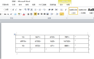 Do you know how to sum a Word table?
Mar 21, 2024 pm 01:10 PM
Do you know how to sum a Word table?
Mar 21, 2024 pm 01:10 PM
Sometimes, we often encounter counting problems in Word tables. Generally, when encountering such problems, most students will copy the Word table to Excel for calculation; some students will silently pick up the calculator. Calculate. Is there a quick way to calculate it? Of course there is, in fact the sum can also be calculated in Word. So, do you know how to do it? Today, let’s take a look together! Without further ado, friends in need should quickly collect it! Step details: 1. First, we open the Word software on the computer and open the document that needs to be processed. (As shown in the picture) 2. Next, we position the cursor on the cell where the summed value is located (as shown in the picture); then, we click [Menu Bar
