Practical tips for excel tables

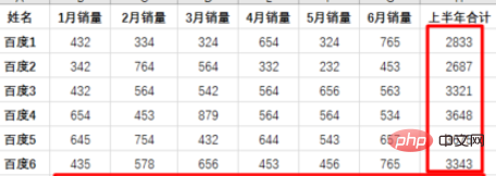
Open the Excel cell, enter the basic data, then we perform a one-second sum, select all the data, hold down "alt =" for one second to find all the sums
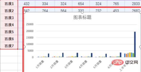
Select all cell data and hold down "alt f1" to create a chart in one second
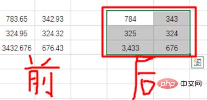
Select the table data, and hold down "ctrl shift 1" at the same time, you can delete the decimal point in the data in one second
Enter splittable long text in the cell, first change the first Row data is split.

Select the data that needs to be split in the first column, and hold down "ctrl E" to split the same text as the first row
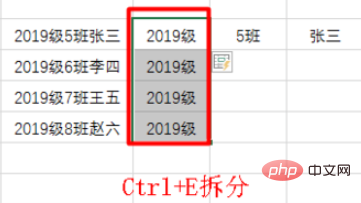
The same applies to the other two columns. After selecting the column, press and hold "ctrl e" to split it

Recommended related article tutorials:excel tutorial
The above is the detailed content of Practical tips for excel tables. For more information, please follow other related articles on the PHP Chinese website!

Hot AI Tools

Undresser.AI Undress
AI-powered app for creating realistic nude photos

AI Clothes Remover
Online AI tool for removing clothes from photos.

Undress AI Tool
Undress images for free

Clothoff.io
AI clothes remover

AI Hentai Generator
Generate AI Hentai for free.

Hot Article

Hot Tools

Notepad++7.3.1
Easy-to-use and free code editor

SublimeText3 Chinese version
Chinese version, very easy to use

Zend Studio 13.0.1
Powerful PHP integrated development environment

Dreamweaver CS6
Visual web development tools

SublimeText3 Mac version
God-level code editing software (SublimeText3)

Hot Topics
 1386
1386
 52
52
 What should I do if the frame line disappears when printing in Excel?
Mar 21, 2024 am 09:50 AM
If when opening a file that needs to be printed, we will find that the table frame line has disappeared for some reason in the print preview. When encountering such a situation, we must deal with it in time. If this also appears in your print file If you have questions like this, then join the editor to learn the following course: What should I do if the frame line disappears when printing a table in Excel? 1. Open a file that needs to be printed, as shown in the figure below. 2. Select all required content areas, as shown in the figure below. 3. Right-click the mouse and select the "Format Cells" option, as shown in the figure below. 4. Click the “Border” option at the top of the window, as shown in the figure below. 5. Select the thin solid line pattern in the line style on the left, as shown in the figure below. 6. Select "Outer Border"
 How to filter more than 3 keywords at the same time in excel
Mar 21, 2024 pm 03:16 PM
Excel is often used to process data in daily office work, and it is often necessary to use the "filter" function. When we choose to perform "filtering" in Excel, we can only filter up to two conditions for the same column. So, do you know how to filter more than 3 keywords at the same time in Excel? Next, let me demonstrate it to you. The first method is to gradually add the conditions to the filter. If you want to filter out three qualifying details at the same time, you first need to filter out one of them step by step. At the beginning, you can first filter out employees with the surname "Wang" based on the conditions. Then click [OK], and then check [Add current selection to filter] in the filter results. The steps are as follows. Similarly, perform filtering separately again
 Steps to adjust the format of pictures inserted in PPT tables
Mar 26, 2024 pm 04:16 PM
1. Create a new PPT file and name it [PPT Tips] as an example. 2. Double-click [PPT Tips] to open the PPT file. 3. Insert a table with two rows and two columns as an example. 4. Double-click on the border of the table, and the [Design] option will appear on the upper toolbar. 5. Click the [Shading] option and click [Picture]. 6. Click [Picture] to pop up the fill options dialog box with the picture as the background. 7. Find the tray you want to insert in the directory and click OK to insert the picture. 8. Right-click on the table box to bring up the settings dialog box. 9. Click [Format Cells] and check [Tile images as shading]. 10. Set [Center], [Mirror] and other functions you need, and click OK. Note: The default is for pictures to be filled in the table
 Where to set excel reading mode
Mar 21, 2024 am 08:40 AM
In the study of software, we are accustomed to using excel, not only because it is convenient, but also because it can meet a variety of formats needed in actual work, and excel is very flexible to use, and there is a mode that is convenient for reading. Today I brought For everyone: where to set the excel reading mode. 1. Turn on the computer, then open the Excel application and find the target data. 2. There are two ways to set the reading mode in Excel. The first one: In Excel, there are a large number of convenient processing methods distributed in the Excel layout. In the lower right corner of Excel, there is a shortcut to set the reading mode. Find the pattern of the cross mark and click it to enter the reading mode. There is a small three-dimensional mark on the right side of the cross mark.
 Practical tips for converting full-width English letters into half-width form
Mar 26, 2024 am 09:54 AM
Practical tips for converting full-width English letters into half-width forms. In modern life, we often come into contact with English letters, and we often need to input English letters when using computers, mobile phones and other devices. However, sometimes we encounter full-width English letters, and we need to use the half-width form. So, how to convert full-width English letters to half-width form? Here are some practical tips for you. First of all, full-width English letters and numbers refer to characters that occupy a full-width position in the input method, while half-width English letters and numbers occupy a full-width position.
 How to set WPS value to automatically change color according to conditions_Steps to set WPS table value to automatically change color according to condition
Mar 27, 2024 pm 07:30 PM
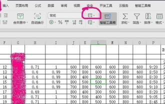
1. Open the worksheet and find the [Start]-[Conditional Formatting] button. 2. Click Column Selection and select the column to which conditional formatting will be added. 3. Click the [Conditional Formatting] button to bring up the option menu. 4. Select [Highlight conditional rules]-[Between]. 5. Fill in the rules: 20, 24, dark green text with dark fill color. 6. After confirmation, the data in the selected column will be colored with corresponding numbers, text, and cell boxes according to the settings. 7. Conditional rules without conflicts can be added repeatedly, but for conflicting rules WPS will replace the previously established conditional rules with the last added rule. 8. Repeatedly add the cell columns after [Between] rules 20-24 and [Less than] 20. 9. If you need to change the rules, you can just clear the rules and then reset the rules.
 How to insert excel icons into PPT slides
Mar 26, 2024 pm 05:40 PM
1. Open the PPT and turn the page to the page where you need to insert the excel icon. Click the Insert tab. 2. Click [Object]. 3. The following dialog box will pop up. 4. Click [Create from file] and click [Browse]. 5. Select the excel table to be inserted. 6. Click OK and the following page will pop up. 7. Check [Show as icon]. 8. Click OK.
 How to read excel data in html
Mar 27, 2024 pm 05:11 PM
How to read excel data in html: 1. Use JavaScript library to read Excel data; 2. Use server-side programming language to read Excel data.


