In an Excel table, when there is a lot of data, it is easy to misread the row and column data. Today I will teach you a cross highlighting technique. When the data point reaches a certain point, the row and column will be automatically highlighted. Don’t worry about reading the wrong data!

How to highlight cross rows and columns in Excel
1. I usually use WPS for making tables
WPS has an advantage in this function. The setting is relatively simple. You only need to activate the reading mode under the view menu bar, and then select a cross color arbitrarily.
Recommended learning: excel basic tutorial
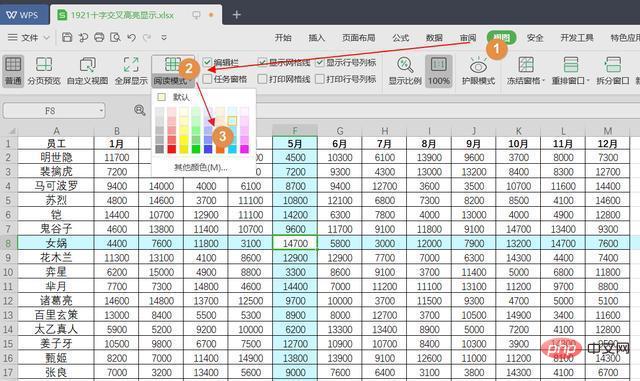
2. OFFICE Excel
The setting in the Excel table is relatively complicated. There are two situations and two methods:
● Suitable for when conditional formatting is not set in the worksheet
We are Under Visual basic of the development tool, or directly press ALT F11

to enter a string of codes in thisbook:

The code is as follows, you can copy and paste it directly. If you need a different color, you only need to change 20 to other numbers
Private Sub Workbook_SheetSelectionChange(ByVal Sh As Object, ByVal Target As Range)
    Cells.FormatConditions.Delete
        With Target.EntireColumn
            .FormatConditions.Add xlExpression, , "=true"
            .FormatConditions(1).Interior.ColorIndex = 20
        End With
        With Target.EntireRow
            .FormatConditions.Add xlExpression, , "=true"
            .FormatConditions(2).Interior.ColorIndex = 20
        End
WithEnd SubThe effect is as follows:
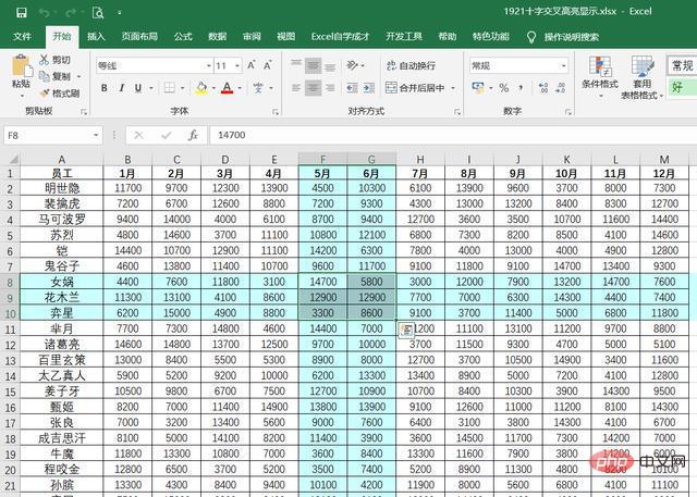
This code is applicable if there is no conditional formatting setting. If it is set, then use the following method
● It is applicable to the worksheet without any cell mark color
Similarly Press ALT F11 in the table, then enter the code:

where the code is:
Private Sub Workbook_SheetSelectionChange(ByVal Sh As Object, ByVal Target As Range)
Sh.Cells.Interior.ColorIndex = xlNone
     Target.EntireColumn.Interior.ColorIndex = 36
     Target.EntireRow.Interior.ColorIndex = 36
End SubThis time we use 36, when we click on the cell , the display effect is yellow, as shown below:
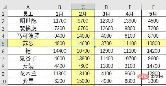
Of course, when there is useful code in the Excel table, you need to save the table as xlsm format

Next time you need to cross-display data, use the above techniques to set it up. Have you learned it? Give it a try~
For more Excel-related tutorials, please pay attention to PHP Chinese website!
The above is the detailed content of How to highlight cross rows in Excel. For more information, please follow other related articles on the PHP Chinese website!
 Compare the similarities and differences between two columns of data in excel
 excel duplicate item filter color
 How to copy an Excel table to make it the same size as the original
 Excel table slash divided into two
 Excel diagonal header is divided into two
 Absolute reference input method
 java export excel
 Excel input value is illegal