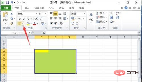
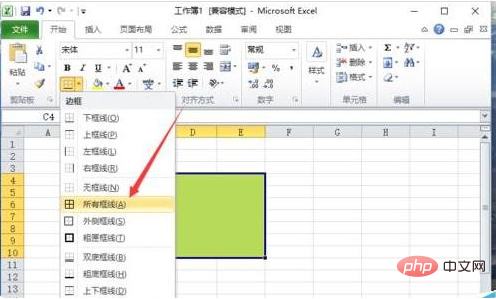
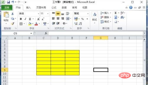
How to display grid lines in Excel: First select the area where you want to add color, click the "Fill Color" option; then click "Lower Border Line" in the "Font" grouping area under the "Start" menu option button; finally select the "All Frames" option.

The operating environment of this article: Windows 7 system, Microsoft Office Excel 2010 version, Dell G3 computer.
How to display grid lines in excel:
1. Double-click the left mouse button on the Excel 2010 workbook program icon on the computer desktop to open and run it. As shown in the figure;

#2. In the open Excel table editing window, select the area where you want to add color. As shown in the picture;

3. Then click the "Fill Color" option and select a color you like to fill. As shown in the picture;

4. Then click the "Underline" button in the "Font" group area under the "Start" menu option. As shown in the picture;

5. Expand all "lines" and select the "all frame lines" option. As shown in the figure;

6. Return to the Excel 2010 worksheet editing window, and you can see that all added color areas have grid lines displayed. As shown in the picture;

Related learning recommendations: excel tutorial
The above is the detailed content of How to display grid lines in excel. For more information, please follow other related articles on the PHP Chinese website!
 Compare the similarities and differences between two columns of data in excel
 excel duplicate item filter color
 How to copy an Excel table to make it the same size as the original
 Excel table slash divided into two
 Excel diagonal header is divided into two
 Absolute reference input method
 java export excel
 Excel input value is illegal


