How to freeze the first three columns of the table in excel: First open an excel table, select the cells in the first three columns; then click "View", "Freeze Panes", and select "Freeze Spaces (F)" and click That’s it.

The operating environment of this article: Windows 7 system, Microsoft Office Excel 2010 version, Dell G3 computer.
How to freeze the first three columns of the table in excel:
1. First, we create or open an excel table.
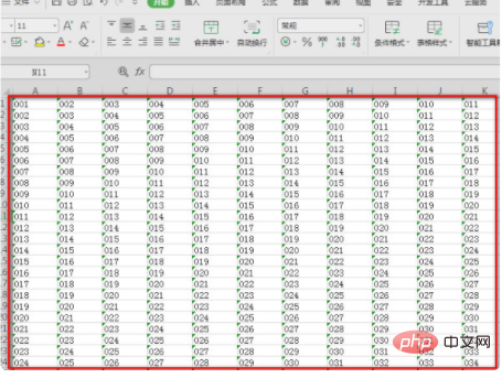
#2. To freeze the first three columns, select the cells in the first three columns as shown in the figure.
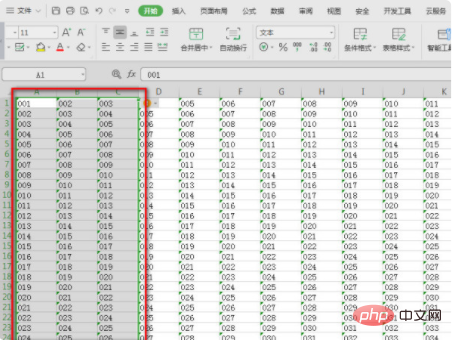
3. After selecting the cells in the first three columns, click "View" - "Freeze Panes" and select "Freeze Spaces (F)" in the frozen panes. Click.

#4. After clicking Finish, as shown in the figure, you can see that the table lines behind the cells in the first three columns turn green, indicating that the first three columns have been frozen.

5. Scroll the mouse to the right. You can see that the first three columns (A, B, C) have not changed, and the following (D) has been moved forward.

Related learning recommendations: excel tutorial
The above is the detailed content of How to freeze the first three columns of excel table. For more information, please follow other related articles on the PHP Chinese website!
 Compare the similarities and differences between two columns of data in excel
 excel duplicate item filter color
 How to copy an Excel table to make it the same size as the original
 Excel table slash divided into two
 Excel diagonal header is divided into two
 Absolute reference input method
 java export excel
 Excel input value is illegal


