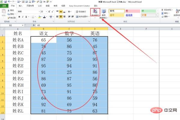
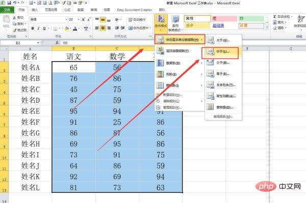
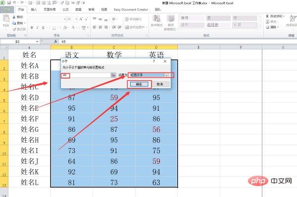
Method: 1. Open the excel table that needs to be operated, select the cells that need to be marked, and select "Conditional Formatting" in the "Home" tab; 2. Click "Highlight Cell Rules" and select " Less than"; 3. Enter "60" in the "Less than" input box, and select "Red Text" in the "Set as" option; 4. Click the "OK" button.

The operating environment of this tutorial: Windows 7 system, Microsoft Office Excel 2010 version, Dell G3 computer.
The steps are as follows:
1. Open the EXCEL table that needs to be operated, select the cells that need to be marked, find the style item on the Home tab, and click "Conditions" Format".

#2. Click "Highlight Cell Rules" and then select "Less Than".

3. Enter "60" in the less than input box, select "Red Text" as the option later, and then click the OK button.

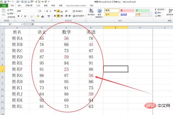
4. Return to the EXCEL table and you will find that the cell text less than 60 is marked in red.

[Recommended learning: Excel tutorial]
The above is the detailed content of How to filter red marks with a score below 60 in excel. For more information, please follow other related articles on the PHP Chinese website!
 Compare the similarities and differences between two columns of data in excel
 excel duplicate item filter color
 How to copy an Excel table to make it the same size as the original
 Excel table slash divided into two
 Excel diagonal header is divided into two
 Absolute reference input method
 java export excel
 Excel input value is illegal