What should I do if N/A appears when using the vlookup function?
Solution: 1. Select the column you want to find, use the "Replace" option to delete all spaces; 2. The first column of the vlookup function must correspond to the column where the value is to be found; 3. Search in the range When using exact search, "#N/A" will appear. In this case, non-exact search method should be used.

The operating environment of this tutorial: Windows 7 system, Microsoft Office Excel 2007 version, Dell G3 computer.
When using the vlookup function in excel, an #N/A error occurs. The main reason is that the corresponding value cannot be found.
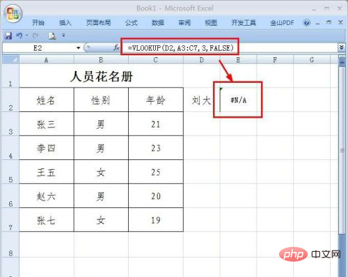
The corresponding value cannot be found, mainly for the following reasons. First, the value being searched is not stored in the search range.
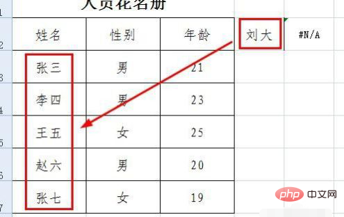
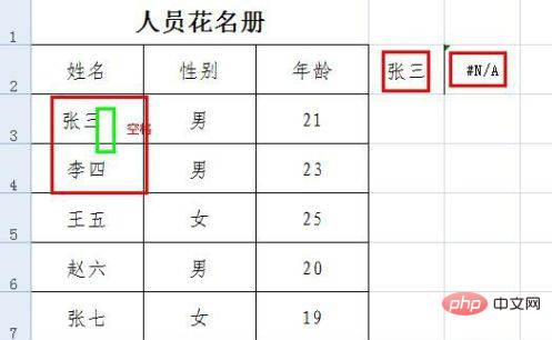
This situation generally occurs when the field includes spaces, which may be at any position. At this time, you can first select the column you want to find, and then use the replace function to delete all spaces.
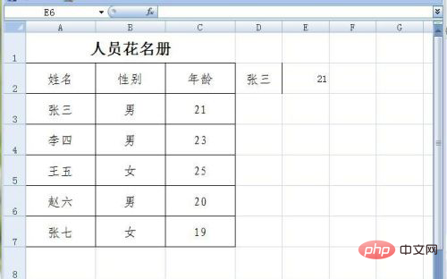
Another reason why the value cannot be found is due to incorrect selection of the search range. In the vlookup function, the first column of the specified range must correspond to the column of the lookup value.
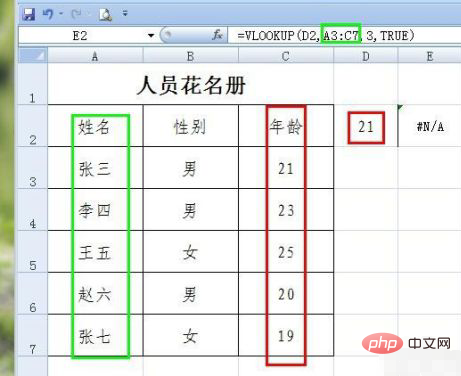
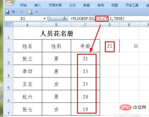
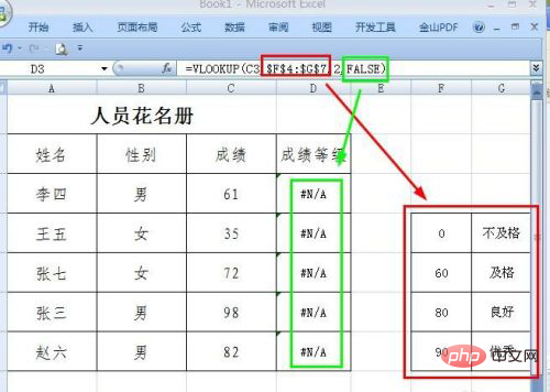
The last situation is caused by inaccurate selection of the search method. For example, if you use precise search during range search, an alarm will be issued. In this case, you should use non-exact search method.
Related learning recommendations: excel tutorial
The above is the detailed content of What should I do if N/A appears when using the vlookup function?. For more information, please follow other related articles on the PHP Chinese website!

Hot AI Tools

Undresser.AI Undress
AI-powered app for creating realistic nude photos

AI Clothes Remover
Online AI tool for removing clothes from photos.

Undress AI Tool
Undress images for free

Clothoff.io
AI clothes remover

AI Hentai Generator
Generate AI Hentai for free.

Hot Article

Hot Tools

Notepad++7.3.1
Easy-to-use and free code editor

SublimeText3 Chinese version
Chinese version, very easy to use

Zend Studio 13.0.1
Powerful PHP integrated development environment

Dreamweaver CS6
Visual web development tools

SublimeText3 Mac version
God-level code editing software (SublimeText3)

Hot Topics
 What does graphics card temperature n/a mean?
Mar 04, 2024 am 09:55 AM
Many users will find that n/a is displayed when they check the graphics card related data of their computers. Many users do not know what this display means. In fact, the main meaning is not applicable. What does graphics card temperature n/a mean? Answer: It means not applicable. The heat dissipation method is natural air cooling 1. The ID of the GPUGPU, which corresponds to 0 and 1, indicating that the IDs of the two GPUs are 0 and 1 respectively; 2. NameGPU name 3. Persistence-M (PersistenceMode) allows the GPU to respond faster Task and standby power consumption increase. Off by default; 4. Fan fan speed (0%–100%), N/A means no fan; 5. Temp graphics card temperature, (GPU temperature is too high
 Parameters of vlookup function and explanation of their meanings
Jan 09, 2024 pm 03:18 PM
We must have used the vlookup function when using excel. So there are several such functions, and how each function is used. As far as the editor knows, there are four vlookup functions, namely Lookup_value, Table_array, col_index_num, and Range_lookup. So let me tell you their specific usage~ The vlookup function has several parameters and the meaning of each parameter. The parameters of the vlookup function include Lookup_value, Table_array, col_index_num, and Range_lookup, a total of 4. 1.Lookup
 How to use vlookup function to match across tables
Feb 20, 2024 pm 11:30 PM
The vlookup function is one of the most commonly used functions in Excel. It can help us find a specified value in a table and return the corresponding value in another table that matches the value. In this article, we will explore the use of the vlookup function, especially when performing cross-table matching. First, let's learn the basic syntax of the vlookup function. In Excel, the syntax of the vlookup function is as follows: =vlookup(lookup_value,ta
 An error occurred when using the vlookup function
Feb 21, 2024 pm 12:18 PM
The vlookup function is a very commonly used search function in Excel. It is used to find a value in a specified data range and return its corresponding data. However, many people may encounter some errors when using the vlookup function. This article will introduce some common vlookup function usage errors and provide solutions. Before using the vlookup function, you first need to understand its syntax. The syntax of the vlookup function is as follows: =VLOOKUP(lookup_value,ta
 How to use formula vlookup
Feb 19, 2024 pm 10:37 PM
The formula VLOOKUP is a very commonly used function in Microsoft Excel. It is used to find a specific value in a table or data set and return other values associated with it. In this article, we will learn how to use the VLOOKUP formula correctly. The basic syntax of the VLOOKUP function is as follows: VLOOKUP(lookup_value, table_array, col_index_num, [range_lookup]) where: lookup
 How to use the vlookup function-How to use the vlookup function
Mar 04, 2024 pm 12:31 PM
Many friends don't know how to use the vlookup function, so the editor will share how to use the vlookup function below. Let's take a look. I believe it will be helpful to everyone. 1. Accurate search According to the accurate information, query the corresponding data in the data table. In the figure, you can search the student ID by name and use "=VLOOKUP(F3,A1:D5,4,0)". 2. Multi-condition search If there are duplicate data in the table, you need to add conditions to limit the query. The formula used to find Class 2 Li Bai in the picture is "=VLOOKUP(F5&G5,IF({1,0},A3:A11&B3:B11,D3:D11),2,FALSE)". 3. For reverse lookup, we want to use VLOOK
 Application of VLOOKUP function in Excel function formula
Mar 20, 2024 am 11:30 AM
There are many function formulas, but not all of them are easy to use. In the past, I preferred to use index and match to achieve what Vlookup can do. But after I really got to know the Vlookup family, I decided to use index and match. Instead of using the Vlookup function, I will now introduce the Vlookup function formula to the readers in detail. First we need to enter the formula =Vlookup(H1, conditional area, return the number of area columns, precise or approximate), where H1 is the position of the red rose. After that, we will add the formula. How to choose this conditional area? This area requires the condition to be in the first column, which is the column with the color of our red rose. It must be this
 Steps to use the VLOOKUP function
Feb 19, 2024 pm 03:54 PM
The vlookup function is a very commonly used function in Excel and plays an important role in data processing and analysis. It can search for matching values in a data table based on specified keywords and return corresponding results, providing users with the ability to quickly find and match data. The following will introduce the use of the vlookup function in detail. The basic syntax of the vlookup function is: =VLOOKUP(lookup_value,table_array,col_index


