The basic functions of excel are: 1. SUM, used for summing, the syntax "sum(value 1, value 2...)"; 2. AVERAGE, used to calculate the average, the syntax "AVERAGE (value 1, value 2...)"; 3. count, used to calculate the number of cells, the syntax is "COUNT (value 1, value 2...)" and so on.

The operating environment of this tutorial: Windows 7 system, Microsoft Office Excel 2016 version, Dell G3 computer.
excel basic functions
1. SUM function: The function of the SUM function is to sum. Syntax: sum(Number 1,Number 2...)
For example: Count a cell range: =sum(A1:A10) Count multiple cell ranges: =sum( A1:A10,C1:C10)
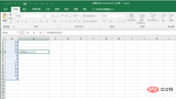
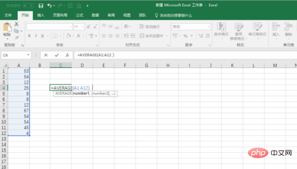
2. AVERAGE function: The function of Average is to calculate the average. Syntax: AVERAGE(Number 1,Number 2...)
For example: Calculate the average of multiple cells =AVERAGE(A1:A12)
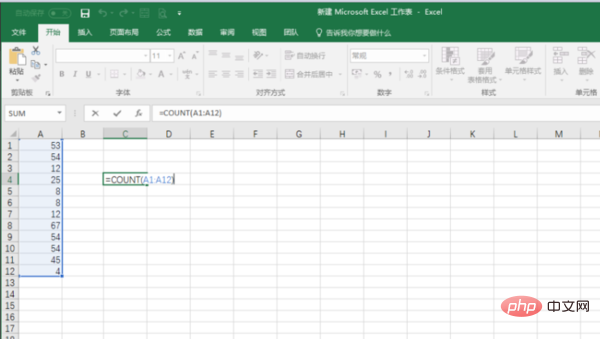
3. Count function: Its function is to count the number of cells. Syntax: COUNT(value 1, value 2...)
For example =COUNT(A1:A12)
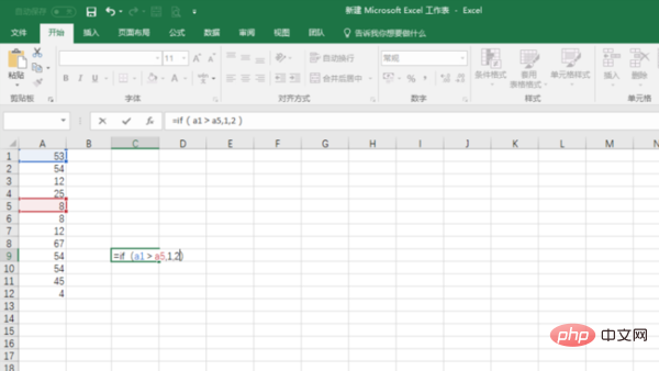
4, IF function: IF function Its function is to judge a condition and then return the specified value based on the result of the judgment.
IF function formula is: =IF (logical judgment, the result when it is TRUE, the result when it is FALSE)
For example: the given condition is A1>A5, if the comparison result is TRUE, then the IF function returns the value of the second parameter; if it is FALSE, it returns the value of the third parameter. =IF(A1>A5,1,2)
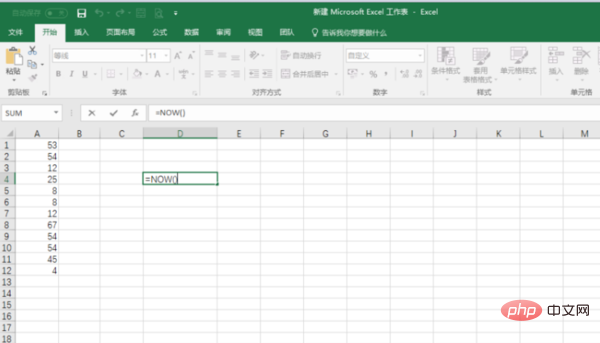
5. NOW function and TODAY function: NOW function returns date and time. The TODAY function only returns the date.
NOW function and TODAY function have no parameters, just use a pair of brackets: =NOW()=TODAY()
Suppose you want to calculate the total number of days a project has been carried out until today. ?=TODAY()-start date, the number obtained is the number of days for the project.
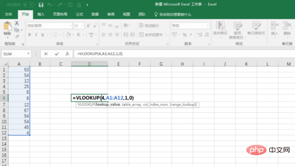
#6. VLOOKUP function: The VLOOKUP function is used to find data in the table.
The syntax formula of the function is: =VLOOKUP(lookup value, area, the content of which column to return, 1 approximate match 0 exact match)
7. Function name: ABS
Main function: Find the absolute value of the corresponding number.
Usage format: ABS(number)
Parameter description: number represents the value or referenced cell whose absolute value needs to be calculated.
Application example: If you enter the formula: =ABS(A2) in cell B2, whether you enter a positive number (such as 100) or a negative number (such as -100) in cell A2, it will be displayed in B2 Output a positive number (such as 100). Use relative references
Special reminder: If the number parameter is not a numerical value, but some characters (such as A, etc.), the error value "#VALUE!" will be returned in B2.
8. Function name: AND
Main function: Return logical value: If all parameter values are logical "TRUE", then return logical "TRUE", otherwise return logical "FALSE".
Usage format: AND(logical1,logical2,...)
Parameter description: Logical1,Logical2,Logical3...: Indicates the condition value or expression to be tested, up to 30 of these .
Application example: Enter the formula in cell C5: =AND(A5>=60,B5>=60) and confirm. If TRUE is returned in C5, it means that the values in A5 and B5 are both greater than or equal to 60. If FALSE is returned, it means that at least one of the values in A5 and B5 is less than 60.
Special reminder: If the specified logical condition parameter contains a non-logical value, the function returns the error value "#VALUE!" or "#NAME".
9. Function name: AVERAGE
Main function: Find the arithmetic average of all parameters.
Using format: AVERAGE(number1,number2,…)
Parameter description: number1,number2,…: The average value or reference cell (area) needs to be calculated, and the parameter does not More than 30.
Application example: Enter the formula in cell B8: =AVERAGE(B7:D7,F7:H7,7,8). After confirmation, you can find the area from B7 to D7 and F7 to H7. value and the average value of 7 and 8.
Special reminder: If the reference range contains "0" value cells, they will be counted; if the reference range contains blank or character cells, they will not be counted.
10. Function name: COLUMN
Main function: Display the column label value of the referenced cell.
Usage format: COLUMN(reference)
Parameter description: reference is the referenced cell.
Application example: Enter the formula in cell C11: =COLUMN(B11). After confirmation, it will be displayed as 2 (i.e. column B).
Special reminder: If you enter the formula: =COLUMN() in cell B11, 2 will also be displayed; correspondingly, there is a function that returns the row label value-ROW(reference).
11. Function name: CONCATENATE
Main function: Connect multiple character texts or data in cells together and display them in one cell.
Usage format: CONCATENATE(Text1, Text...)
Parameter description: Text1, Text2... are the character text or referenced cells that need to be connected.
Application example: Enter the formula in cell C14: =CONCATENATE(A14,"@",B14,".com"). After confirmation, the characters, @, and B14 in cell A14 can be The characters in the cell and .com are connected into a whole and displayed in cell C14.
Special reminder: If the parameter is not a referenced cell and is in text format, please add double quotes in English to the parameter. If you change the above formula to: =A14&"@"&B14&". com" can achieve the same purpose.
12. Function name: COUNTIF
Main function: Count the number of cells in a certain cell range that meet the specified conditions.
Usage format: COUNTIF(Range,Criteria)
Parameter description: Range represents the cell range to be counted; Criteria represents the specified conditional expression.
Application example: Enter the formula in cell C17: =COUNTIF(B1:B13,">=80"). After confirmation, you can count the values in the cell range from B1 to B13 that are greater than or equal to The number of cells is 80.
Special reminder: Blank cells are allowed to appear in the referenced cell range.
Related learning recommendations: excel tutorial
The above is the detailed content of What are the basic functions of excel?. For more information, please follow other related articles on the PHP Chinese website!
 Compare the similarities and differences between two columns of data in excel
 excel duplicate item filter color
 How to copy an Excel table to make it the same size as the original
 Excel table slash divided into two
 Excel diagonal header is divided into two
 Absolute reference input method
 java export excel
 Excel input value is illegal


