A brief analysis of the usage of sumif() and countif() in Excel function learning

When we use Excel to create tables to organize data, we use its built-in functions to assist operations, which can improve operational efficiency. Today we will learn how to use Excel functions. Let’s first learn about the application of sumif and countif functions. I hope it will be helpful to everyone!

Part 1: How to use the sumif function

The Sumif function is to specify a pair based on given conditions Cell sum.

First of all, we use a simple data to understand how to use the Sumif function. The picture below is a worksheet source data.

Use the SUMIF function to find the cells in column A that are greater than 15, and sum them with their corresponding cells in column B.

Enter in the evaluation cell: =SUMIF(A1:A4,">15",B1:B4), and the result is 900.

The meaning of the formula is that because the data in A2, A3, and A4 meet the condition ">15", the corresponding data in B2, B3, and B4 are summed and calculated.

The syntax of the SUMIF function is: SUMIF(range,criteria,sum_range)

The parameters are introduced as follows:

• First, range: is the range of cells to be calculated based on conditions. Cells in each range must be numbers and names, arrays, and references containing numbers. Empty values ​​and text values ​​are ignored.

• Second, Criteria: The conditions for determining which cells to add, which can be in the form of numbers, expressions or text. For example, the condition could be expressed as 65, "65", ">65", or "apples".

• Third, Sum_range: is the actual cells to be added (if the relevant cells in the range meet the conditions). If sum_range is omitted, cells in the range are both evaluated conditionally and added when they match the condition.

Sumif function supports wildcard calculation. You can use wildcard characters, question marks (?), and asterisks (*) in criteria. A question mark matches any single character; an asterisk matches any string of characters. If you want to find an actual question mark or asterisk, type a tilde (~) before the character.

Part 2: Application case analysis of sumif function and COUNTIF function

First question: The SUMIF function is used to find And, the COUNTIF function is used for counting. Use these two functions for summation and counting applications respectively.

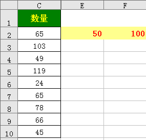
#1. Column C of the following worksheet is the source data. Find the number greater than 50 and less than 100.

The formula is: =COUNTIF($C2:$C10,">"&E2)-COUNTIF(C2:C10," >"&F2), the result is 4.

You can also nest the SUM function to calculate, the formula is: =SUM(COUNTIF(C2:C10,{">50",">=100"})*{1,-1} ).

2. Find the sum greater than 50 and less than 100.

For summation, we only need to replace COUNTIF in the above formula with the sumif function.

The formula is: =SUMIF($C2:$C10,">"&E2)-SUMIF(C2:C10,">"&F2), the result is: 274 .

Or use the array formula: =SUM(COUNTIF(C2:C10,{">50",">=100"})*{1,-1}), three keys to end.

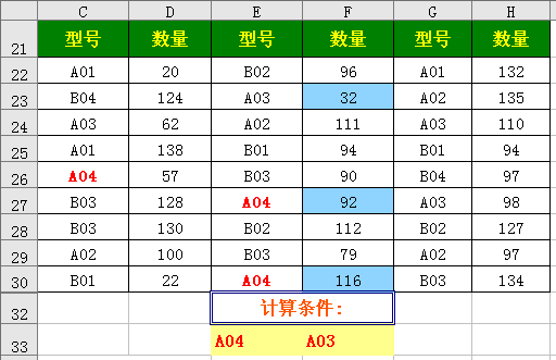
Second question: The picture below is a source data, E33, F33 are calculation conditions, complete the following questions.

1. Find the sum of the quantities corresponding to the cell values ​​of model A04 and A03.

You can apply sumif (area, condition, summation area), and the formula is: =SUMIF(C22:G30,E33,D22:H30) SUMIF(C22:G30,F33,D22: H30), the result is: 745.

Or use the array formula: =SUM(SUMIF(C22:G30,E33:F33,D22)), end with three keys.

2. Find the quantity corresponding to the cell values ​​of models A04 and A03.

The basic principle of finding the number is the same as that of summation, but the functions are different. Therefore the formula is: =COUNTIF(C22:H30,E33) COUNTIF(C22:H30,F33)

or use the array formula =SUM(COUNTIF(C22:G30,E33 :F33)), three keys to end.

3. Find the sum of the quantity of products whose model numbers start with A but do not include A03.

Both the SUMIF and COUNTIF functions support wildcard characters, and you can use wildcard characters, question marks (?) and asterisks (*) in conditions. A question mark matches any single character; an asterisk matches any string of characters. If you want to find an actual question mark or asterisk, type a tilde (~) before the character.

Formula analysis:

Use the SUMIF function to find the total quantity starting with A. The formula is: =SUMIF(C22:G30,F33,D22), and then subtract the value of A03 from this value to get the value other than A03.

The formula is: =SUMIF(C22:G30,"A*",D22)-SUMIF(C22:G30,F33,D22), and the result is: 998.

Related learning recommendations: excel tutorial

The above is the detailed content of A brief analysis of the usage of sumif() and countif() in Excel function learning. For more information, please follow other related articles on the PHP Chinese website!