Let's talk about Excel's SUMPRODUCT function

This article brings you relevant knowledge about excel, which mainly introduces the related issues of the SUMPRODUCT function. This function not only integrates the two major functions of conditional summation and counting, but also It can be used for ranking processing in complex scenarios. Let’s take a look at it. I hope it will be helpful to everyone.

Related learning recommendations: excel tutorial

Today I will share with you a very commonly used and practical function: SUMPRODUCT. As we all know, conditional summation and counting are the two most common problems encountered by table users, and this function not only combines the two major functions of conditional summation and counting; it can also be used for ranking processing in complex scenarios, and even heard that Some people have conquered half of the Excel world with just one function...so they have to learn it.

Basic syntax

Let’s look at the basic syntax first. The official syntax description of SUMPRODUCT is to add the corresponding elements between the arrays in given sets of arrays. Multiply and return the sum of the products. The syntax format is as follows:

=SUMPRODUCT（array1,array2,array3, …）

- SUM means summation, PRODUCT means multiplication. The parameters are multiplied and then summed. You see, SUMPRODUCT does exactly what its name suggests.

Look at my hand, Wai, Tu, Sri... To sum up, the SUMPRODUCT function has the following three characteristics:

1> It performs array operations by default.

2> It will treat non-numeric array elements in the parameters as 0.

3> The parameters must have the same size, otherwise an error value will be returned.

Characteristic Analysis

After reading SUMPRODUCT’s resume, many friends must be looking at it in the fog and only have a vague understanding of it. What do these characteristics of it mean? What kind of work can it do? In fact, it is not clear.

Snap your fingers and let me give you a few examples.

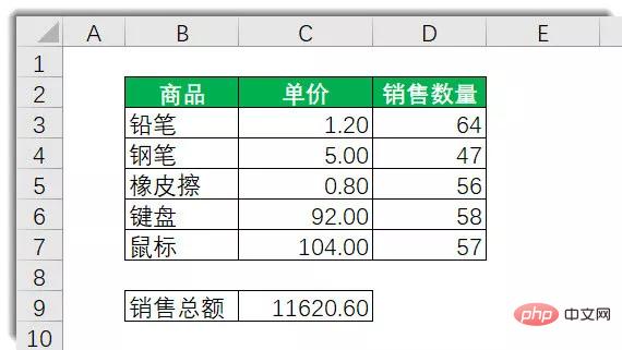
As shown in the data table above, column C is the unit price of the product, and column D is the sales quantity. Now we need to calculate the total sales in cell C9.

C9 Enter the following formula to get the result 11620.60

=SUMPRODUCT(C3:C7, D3:D7)

This is a simple SUMPRODUCT function. Its operation process is: multiply the elements in the two area arrays C3:C7 and D3:D7 respectively, that is, C3*D3, C4*D4, C5*D5... until C7*D7

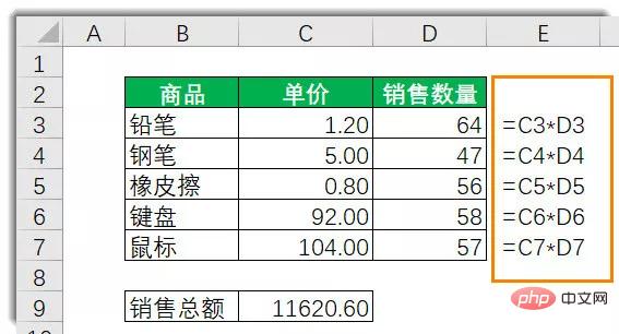
It means first calculating the sales amount of each product, and finally summing it up.

Because the first feature of the SUMPRODUCT function is that it supports operations between arrays, although the formula performs multiple operations, there is no need to press the triple array key to end the formula input.

Some friends said that the formula can also be written like this:

=SUMPRODUCT(C3:C7*D3:D7)

Or you can use the following array formula.

=SUM(C3:C7*D3:D7)

So what are the differences between these three formulas?

First of all, in most cases, the SUMPRODUCT function does not require the array triple key to end the formula input to perform array operations, but the SUM function does.

Secondly, let’s talk about another very important feature of the SUMPRODUCT function.

......

We have slightly changed the above table and changed the sales quantity of "pens" to: Not yet counted. It is also necessary to calculate the total sales in cell C9.

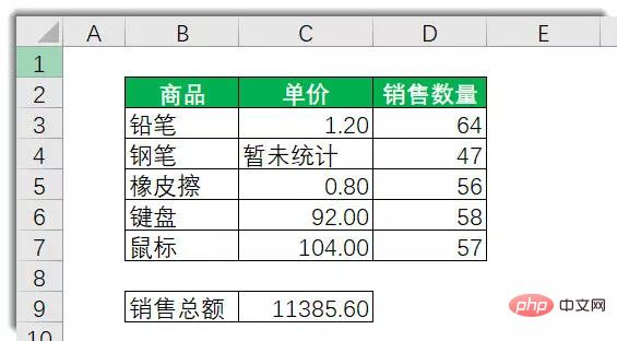
At this time, if you use the formula:

=SUMPRODUCT(C3:C7*D3:D7)

or the array formula:

=SUM(C3:C7*D3:D7)

, the error value #VALUE!## will be returned.

#The reason for returning the error value is that cell D4 is "not yet counted" as a text value. Text values ​​cannot directly participate in mathematical operations, so C4*D4 returns the error value #VALUE!, which in turn causes the result of the entire formula to be returned. Error value.

There is no such problem when using the following formula, and the correct result will be returned directly:

=SUMPRODUCT(C3:C7,D3:D7)

This is SUMPRODUCT The second feature of the function: treat non-numeric array elements as 0.

Take this example, the value of cell D4 "not yet counted" is text, not a numerical value. SUMPRODUCT actively treats it as zero, so C4*D4, the result is also zero, and the other array elements are as usual Calculate and get the result of 11385.60.

It should be noted that SUMPRODUCT treats non-numeric array elements as 0. The so-called non-numeric array elements include logical values ​​and text, but do not contain error values. If the array element contains Error value, the formula also returns an error value, such as the first formula in this example.

……

After talking about the two features of the SUMPRODUCT function, let’s talk about its third feature: the array parameters must have the same size, otherwise an error value will be returned.

We still use the example in the above picture as an example to continue to calculate the total sales of the product. If we enter the formula in C9:

=SUMPRODUCT(C3:C7,D3:D6)

, what will the result be?

Error value: #VALUE!

Why?

细心的你肯定已经注意到了，两个区域数组，C3:C7明显显比D3:D6多了一个元素，C3和D3结对子，C4和D4结对子……那么C7和谁结对子呢？女人们都嫁了，结果剩下一个光棍，这日子没法过了！一个萝卜一个坑，只有萝卜没有坑，这不是要萝卜死吗？

——于是SUMPRODUCT就不高兴了，它给你一个错误值#VALUE!，明确告诉你，和谐时代幸福岁月，日子不能这么过。

这就是SUMPRODUCT函数的第三个特点：数组参数必须有相同的尺寸，否则返回错误值。

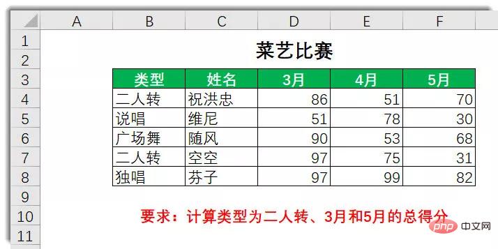
下面是一道练习题，你看看，能用SUMPRODUCT函数做出来吗？

案例拓展

假设下面这张图，是某个公司工资发放的部分记录表（数据纯属虚拟，如有雷同，那是穿越）。A列是工资发放的时间，B列是员工所属的部门，C列是员工姓名，D列是相关员工领取的工资金额。

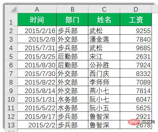
——那么，问题和广告都来了：

1

员工西门庆领取了几次工资？

这是一个单条件计数的问题,通常我们使用COUNTIF函数,但如果使用SUMPRODUCT函数，一般写成这样：

=SUMPRODUCT((C2:C13="西门庆")*1)

先判断C2:C13的值是否等于”西门庆”，相等则返回TRUE，不等则返回FALSE，由此建立一个有逻辑值构成的内存数组。

上文已经说过，SUMPRODUCT有一个特性，它会将非数值型的数组元素作为0处理，逻辑值自然是属于非数值型的数组元素，为了避免SUMPRODUCT函数把逻辑值视为0，造成统计错误，我们使用*1的方式，把逻辑值转化为数值，TRUE转化为1，FALSE转化为0，最后统计求和。

2

员工西门庆领取了多少工资？

这是一个单条件求和的问题,通常我们使用SUMIF函数,如果使用SUMPRODUCT函数，我们可以写成这样：

=SUMPRODUCT((C2:C13="西门庆")*D2:D13)

依然首先判断C2:C13的值是否等于”西门庆”，得到逻辑值FALSE或TRUE，再和D2:D13的值对应相乘。TRUE乘以数值，得到数值本身。FALSE乘以数值返回0。最后统计求和得出结果。

看完了上面两个问题，有些朋友可能会在心里想，貌似SUMPRODUCT能干的事，SUMIF和COUNTIF也能做到，而且做的更好，那么还要SUMPRODUCT干啥嘞？

乡亲们呐，话不能这么说，SUMPRODUCT可是上得厅堂下得厨房，对工作环境不挑不拣，它对参数类型没有啥特别要求，COUNTIF和SUMIF就不同了，他俩要求个别参数，必须是区域（Range型），不支持数组，比如下面这两个问题，COUNTIF和SUMIF就要绕了。

3

二月份外交部发放了几次工资？总额是多少？

第1个问题，二月份外交部发放了几次工资？

这是一个多条件计数的问题。

第一个条件，发放工资的时间必须是二月份；第二个条件，发放工资的部门必须是外交部。

如果使用多条件计数函数COUNTIFS，判断发放工资的时间是否属于六月份，会简单问题复杂化。而使用SUMPRODUCT函数，咱们可以把公式写成这样：

=SUMPRODUCT((MONTH(A2:A13)=2)*(B2:B13="外交部"))

……

第2个问题，统计二月份外交部发放了多少工资？

这是一个常见的多条件求和问题。

如果使用SUMIFS函数，判断发放工资的时间是否属于六月份，也会简单问题复杂化。

SUMPRODUCT跃然而至：

=SUMPRODUCT((MONTH(A2:A13)=6)*(B2:B13="外交部"),D2:D13)

或者：

=SUMPRODUCT((MONTH(A2:A13)=6)*(B2:B13="外交部")*D2:D13)

打个响指，关于这两个形式的SUMPRODUCT函数的区别，咱们上文已有详细说明——你还记得吗？

上面这个公式可以说是SUMPRODUCT多条件求和的典型用法啦，可以归纳为:

=SUMPRODUCT((条件一)*(条件二)……,求和区域)

4

二月份外交部和步兵部合计发放了多少工资？

解决了上面的问题，相信大家已经晓得如何计算二月份外交部发放多少工资了，那么二月份外交部和步兵部合计发了多少工资，又当怎么计算呢

我们经常见有些性格朴素的表亲们把公式写成这样：

=SUMPRODUCT((MONTH(A2:A13)=2)*(B2:B13="外交部")*D2:D13)+SUMPRODUCT((MONTH(A2:A13)=2)*(B2:B13="步兵部")*D2:D13)

这些表亲们估计心想，不就是计算两个部门吗？甭说两个，二十个咱也能算，一个加一个，一直加到二十个，世上无难事，只怕有心人嘛，一砖加一砖，长城就建成了，一泡加一泡，长江就奔流了……

呃……公式写的那么长，先不谈计算速度，首先它累手啊，万一写错了，又要修改，那也是麻烦他妈哭麻烦——麻烦死了。

其实我们可以写成这样：

=SUMPRODUCT((MONTH(A2:A13)=6)*(B2:B13={"外交部","步兵部"})*D2:D13)

5

排名应用

认识了SUMPRODUCT函数在条件计数和求和方面的用法，最后，咱们再来看一个它在排名上的使用方法。

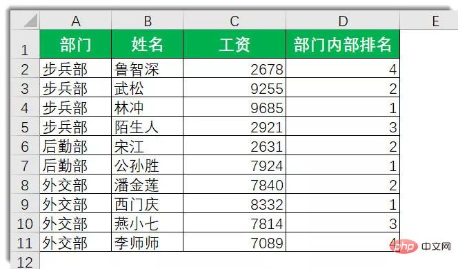
如上图所示，某个月某个公司某些人领了某些工资，然后呢，他们想看看自己的工资，在部门内的排名情况，比如说步兵部的鲁智深都是老员工了，非常想知道自个工资在各自部门排几号。

当然啦，不排不知道，一排就傻掉。

SUMPRODUCT是这么解决这个问题的，D2输入公式向下复制：

=SUMPRODUCT(($A$2:$A$9=A2)*(C2<$C$2:$C$9))+1

（思考，为什么公式的最后+1，而不是直接写成如下：）

=SUMPRODUCT(($A$2:$A$9=A2)*(C2<=$C$2:$C$9))

结束语

唠唠叨叨说了这么多，眼睛都说酸麻了，是到了该结束的时候啦。

最后，请思考两个小问题：

第1个问题：下面SUMPRODUCT函数有几个参数？

=SUMPRODUCT((MONTH(A2:A13)=6)*(B2:B13="财务部")*D2:D13)

下面这个SUMPRODUCT函数又有几个参数？

=SUMPRODUCT((MONTH(A2:A13)=6)*(B2:B13="财务部")，D2:D13)

第二个问题：

SUMPRODUCT为什么有时候比SUMIF/COUNTIF计算速度慢？

相关学习推荐：excel教程

The above is the detailed content of Let's talk about Excel's SUMPRODUCT function. For more information, please follow other related articles on the PHP Chinese website!