In the previous article "How to Filter Excel Pivot Table Learning", we learned the filtering skills of Excel Pivot Table. Today we continue to learn Excel Pivot Tables and explain the date combinations in Pivot Tables. I hope it will be helpful to everyone!

In order to facilitate viewing and statistical data, sometimes we need to group the date fields in the row area. The default combination step size of the date field includes year, month, quarter, and day.
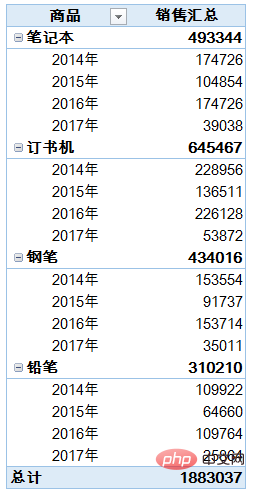
The case of this article is the sales detailed list of a stationery company. In order to analyze revenue, you need to use a pivot table to display the annual cumulative sales of different products. The final pivot table rendering is as follows:

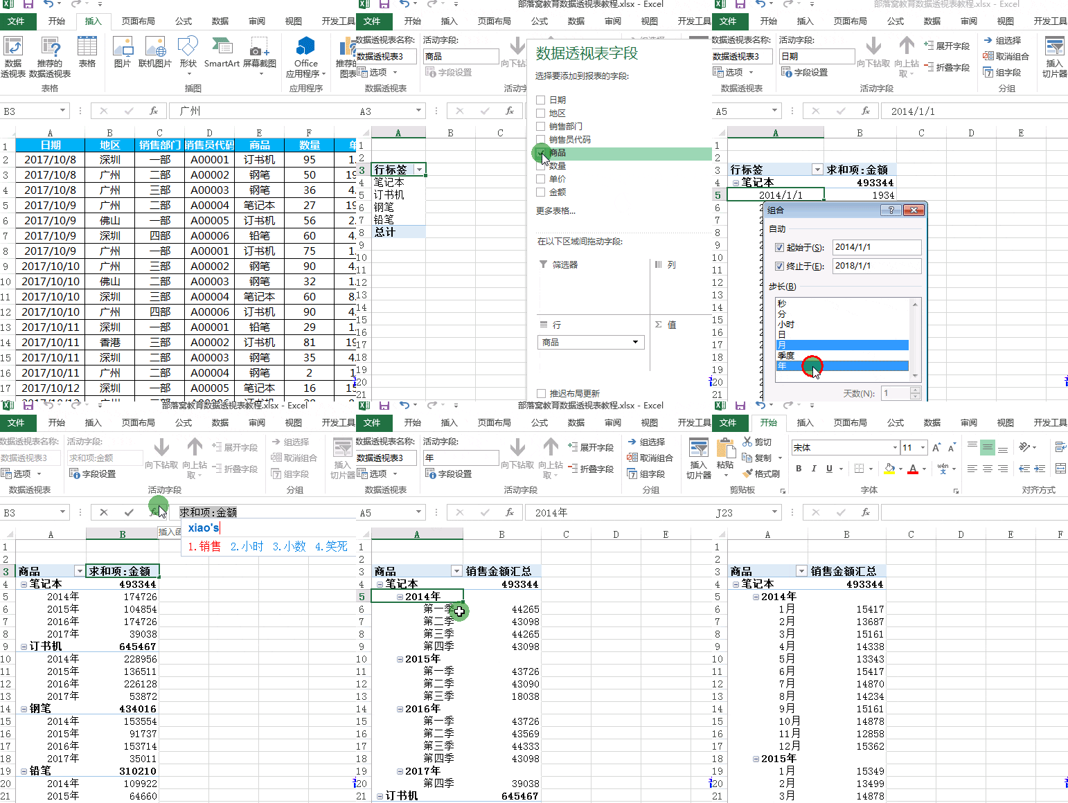
##Knowledge point 1: Year, quarter, month combination
In the pivot table, first Select the date, right-click - Group, you can display it by year, quarter or month. If you want to cancel the date combination, just select the date field, right-click - Ungroup.
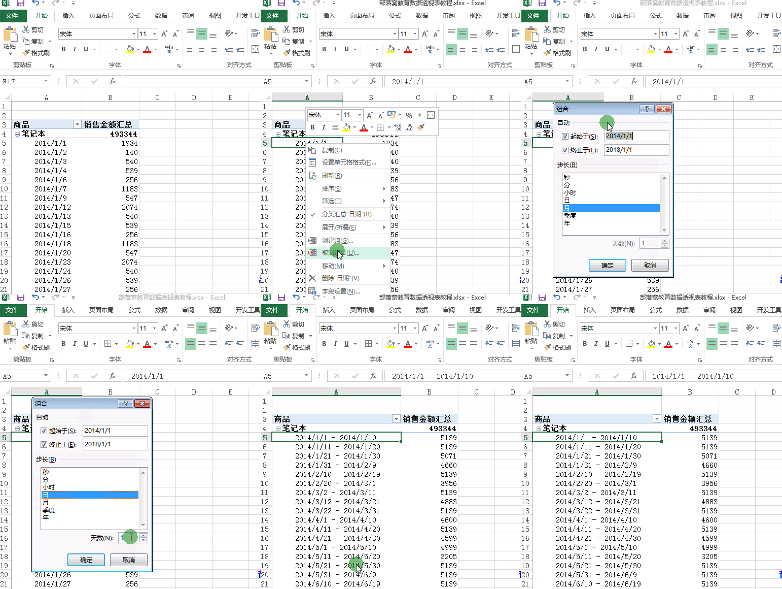
Knowledge point 2: Combination by day
If you want to count the sales every 10 days, first cancel the month, quarter, Year combination, then check the day, and then set the number of days to 10.
The above is the detailed content of Excel pivot table learning how to combine dates. For more information, please follow other related articles on the PHP Chinese website!
 Compare the similarities and differences between two columns of data in excel
 excel duplicate item filter color
 How to copy an Excel table to make it the same size as the original
 Excel table slash divided into two
 Excel diagonal header is divided into two
 Absolute reference input method
 java export excel
 Excel input value is illegal