

Practical Excel skills sharing: Use 'Find and Replace' to filter date data

In the previous article "Practical Excel skills sharing: cleverly using functions to create an automatic statistical inventory table", we learned four functions and used them to make an automatic statistical inventory The purchase, sale, inventory and warehouse statistics table. Today we will share some practical operations of "find and replace". It turns out that you can use it to filter date data. Let's take a look!
When setting the date to filter, how can you filter by year and month? Let’s answer this question today.
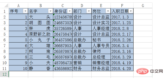
As shown in the figure below, column F is the employee’s entry date, but the date at this time is not in the standard date format. The default standard date format in excel is "-" "/" or the Chinese "year and month" "day" to separate the year, month and day numbers. At this time, I want to filter the table to select employees who joined the company in February 2018.
First add a filter button to the table (Start-Data-Filter). In the drop-down menu of entry date, the data is not divided by year and month. At this point we need to convert the date into a standard date format.

Press ctrl H to replace the shortcut key. In the pop-up dialog box, enter a period in English format for "Find content" and enter "/" in English format for "Replace with" or"-". After setting, click Replace All.
You can now see the replacement results, and all dates have become standard date formats.
Click the drop-down button of the entry date, and you can see that the date is divided into years and months. Click the " " and "-" in front of the number to expand and collapse the data.
We check 2018 and February in the drop-down menu to see the filtering results.

Expand knowledge: Two practical techniques for "find and replace"
1. Batch deletion of invisible characters
When there are a large number of the same characters in our table that need to be deleted, or when we have several worksheets in a workbook that all need to delete the same data, if we have one Deleting it alone is a waste of time. At this time, you need to use the find and replace tool.
As shown in the figure below, sum the F, G, and H columns in Table 1, Table 2, and Table 3. The total salary payable in column H displays 0. When the function operation result is 0, it means that the cell content referenced in the function is not a number. In addition, the number in column H is to the left (if the left-aligned format is removed, it is still to the left), which means it is text type. number.
(Friends who don’t know the shortcut for summation can read the previously published tutorial and click on the link: https://www.php.cn/topic/excel/491692.html)

Let’s first check what went wrong with the data.
Select cell H2 and drag the mouse to select the number in the edit bar. You can see that there are invisible characters in front and behind the number (if there are no characters, dragging the mouse will not select it. If it is selected, it means There are non-whitespace invisible characters). This is what often happens when people export data from the system or copy text from the Internet. Even if the format is cleared, the sum still cannot be added.
Let’s talk about the solution.
In the edit bar, select the invisible characters and press "ctrl C" to copy.
Press the find and replace shortcut key ctrl H to pop up the replacement dialog box. Press "ctrl V" in "Find Content" to copy invisible characters. At this point you can see that the mouse cursor has moved a few spaces to the right.

Do not enter any characters after "Replace with" to indicate that the search content will be deleted. Click the "Scope" drop-down menu to select a workbook. At this time, you can find and replace all worksheets in the entire workbook. Click "Replace All".

At this time, you can see that the data in column H automatically displays the summation result.

Sharp-eyed friends may find that the data is still on the left. This is because left alignment is set in the alignment. We click "Left Alignment" again in the alignment. "Cancel the "left-aligned" format.
At this time, if you look at the tables in Table 2 and Table 3, you will find that all invisible characters have been deleted simultaneously, and the correct result of the total is automatically displayed. .
#2. Batch replacement cell format
In the table below, due to the good performance of Nobita and Shizuka that month, the boss said They wanted to increase their wages individually, so the finance department made a special cell format for their names. The next month, the table needed to be restored to a unified format. The following case mainly talks about batch replacement of color formats. In addition, various cell formats can be replaced in batches.
Press the replacement shortcut key ctrl H. In the pop-up dialog box, click the format drop-down button. At this time, you can see that there are two options available.

When we know the format of the cell, click the first option "Format" and select the corresponding color in the pop-up frame.

When we are not very clear about the format of the cell, click the second option "Select format from cell", and the mouse will turn into a straw. Tool that can directly absorb the color of cells. Here I will directly absorb the color of B7 or B11. You can now see a preview of the color.

The following "Replace with" settings are the same as before. Select the second item "Select format from cell" in the format drop-down menu and absorb any blue cell. Just click the grid. At this point you can see the results below.

If we have multiple worksheets that need to be replaced, just select the workbook in the "Scope" drop-down menu. After setting up, click "Replace All" and you will see that the table changes to a unified color format.

Note: The "Find and Replace" dialog box will remember the last format set, so you need to select "Format" when using Find and Replace again. The "Clear Lookup Formatting" option in the drop-down menu clears the formatting.

Related learning recommendations: excel tutorial
The above is the detailed content of Practical Excel skills sharing: Use 'Find and Replace' to filter date data. For more information, please follow other related articles on the PHP Chinese website!

Hot AI Tools

Undresser.AI Undress
AI-powered app for creating realistic nude photos

AI Clothes Remover
Online AI tool for removing clothes from photos.

Undress AI Tool
Undress images for free

Clothoff.io
AI clothes remover

Video Face Swap
Swap faces in any video effortlessly with our completely free AI face swap tool!

Hot Article
Hot Tools

Notepad++7.3.1
Easy-to-use and free code editor

SublimeText3 Chinese version
Chinese version, very easy to use

Zend Studio 13.0.1
Powerful PHP integrated development environment

Dreamweaver CS6
Visual web development tools

SublimeText3 Mac version
God-level code editing software (SublimeText3)
Hot Topics
 1389
1389
 52
52

 What should I do if the frame line disappears when printing in Excel?
Mar 21, 2024 am 09:50 AM
What should I do if the frame line disappears when printing in Excel?
Mar 21, 2024 am 09:50 AM
If when opening a file that needs to be printed, we will find that the table frame line has disappeared for some reason in the print preview. When encountering such a situation, we must deal with it in time. If this also appears in your print file If you have questions like this, then join the editor to learn the following course: What should I do if the frame line disappears when printing a table in Excel? 1. Open a file that needs to be printed, as shown in the figure below. 2. Select all required content areas, as shown in the figure below. 3. Right-click the mouse and select the "Format Cells" option, as shown in the figure below. 4. Click the “Border” option at the top of the window, as shown in the figure below. 5. Select the thin solid line pattern in the line style on the left, as shown in the figure below. 6. Select "Outer Border"
 How to filter more than 3 keywords at the same time in excel
Mar 21, 2024 pm 03:16 PM
How to filter more than 3 keywords at the same time in excel
Mar 21, 2024 pm 03:16 PM
Excel is often used to process data in daily office work, and it is often necessary to use the "filter" function. When we choose to perform "filtering" in Excel, we can only filter up to two conditions for the same column. So, do you know how to filter more than 3 keywords at the same time in Excel? Next, let me demonstrate it to you. The first method is to gradually add the conditions to the filter. If you want to filter out three qualifying details at the same time, you first need to filter out one of them step by step. At the beginning, you can first filter out employees with the surname "Wang" based on the conditions. Then click [OK], and then check [Add current selection to filter] in the filter results. The steps are as follows. Similarly, perform filtering separately again
 How to change excel table compatibility mode to normal mode
Mar 20, 2024 pm 08:01 PM
How to change excel table compatibility mode to normal mode
Mar 20, 2024 pm 08:01 PM
In our daily work and study, we copy Excel files from others, open them to add content or re-edit them, and then save them. Sometimes a compatibility check dialog box will appear, which is very troublesome. I don’t know Excel software. , can it be changed to normal mode? So below, the editor will bring you detailed steps to solve this problem, let us learn together. Finally, be sure to remember to save it. 1. Open a worksheet and display an additional compatibility mode in the name of the worksheet, as shown in the figure. 2. In this worksheet, after modifying the content and saving it, the dialog box of the compatibility checker always pops up. It is very troublesome to see this page, as shown in the figure. 3. Click the Office button, click Save As, and then
 How to type subscript in excel
Mar 20, 2024 am 11:31 AM
How to type subscript in excel
Mar 20, 2024 am 11:31 AM
eWe often use Excel to make some data tables and the like. Sometimes when entering parameter values, we need to superscript or subscript a certain number. For example, mathematical formulas are often used. So how do you type the subscript in Excel? ?Let’s take a look at the detailed steps: 1. Superscript method: 1. First, enter a3 (3 is superscript) in Excel. 2. Select the number "3", right-click and select "Format Cells". 3. Click "Superscript" and then "OK". 4. Look, the effect is like this. 2. Subscript method: 1. Similar to the superscript setting method, enter "ln310" (3 is the subscript) in the cell, select the number "3", right-click and select "Format Cells". 2. Check "Subscript" and click "OK"
 How to set superscript in excel
Mar 20, 2024 pm 04:30 PM
How to set superscript in excel
Mar 20, 2024 pm 04:30 PM
When processing data, sometimes we encounter data that contains various symbols such as multiples, temperatures, etc. Do you know how to set superscripts in Excel? When we use Excel to process data, if we do not set superscripts, it will make it more troublesome to enter a lot of our data. Today, the editor will bring you the specific setting method of excel superscript. 1. First, let us open the Microsoft Office Excel document on the desktop and select the text that needs to be modified into superscript, as shown in the figure. 2. Then, right-click and select the "Format Cells" option in the menu that appears after clicking, as shown in the figure. 3. Next, in the “Format Cells” dialog box that pops up automatically
 How to use the iif function in excel
Mar 20, 2024 pm 06:10 PM
How to use the iif function in excel
Mar 20, 2024 pm 06:10 PM
Most users use Excel to process table data. In fact, Excel also has a VBA program. Apart from experts, not many users have used this function. The iif function is often used when writing in VBA. It is actually the same as if The functions of the functions are similar. Let me introduce to you the usage of the iif function. There are iif functions in SQL statements and VBA code in Excel. The iif function is similar to the IF function in the excel worksheet. It performs true and false value judgment and returns different results based on the logically calculated true and false values. IF function usage is (condition, yes, no). IF statement and IIF function in VBA. The former IF statement is a control statement that can execute different statements according to conditions. The latter
 Where to set excel reading mode
Mar 21, 2024 am 08:40 AM
Where to set excel reading mode
Mar 21, 2024 am 08:40 AM
In the study of software, we are accustomed to using excel, not only because it is convenient, but also because it can meet a variety of formats needed in actual work, and excel is very flexible to use, and there is a mode that is convenient for reading. Today I brought For everyone: where to set the excel reading mode. 1. Turn on the computer, then open the Excel application and find the target data. 2. There are two ways to set the reading mode in Excel. The first one: In Excel, there are a large number of convenient processing methods distributed in the Excel layout. In the lower right corner of Excel, there is a shortcut to set the reading mode. Find the pattern of the cross mark and click it to enter the reading mode. There is a small three-dimensional mark on the right side of the cross mark.
 How to insert excel icons into PPT slides
Mar 26, 2024 pm 05:40 PM
How to insert excel icons into PPT slides
Mar 26, 2024 pm 05:40 PM
1. Open the PPT and turn the page to the page where you need to insert the excel icon. Click the Insert tab. 2. Click [Object]. 3. The following dialog box will pop up. 4. Click [Create from file] and click [Browse]. 5. Select the excel table to be inserted. 6. Click OK and the following page will pop up. 7. Check [Show as icon]. 8. Click OK.
