Practical Excel skills sharing: How to extract numbers?
In the previous article "Sharing practical Excel skills: 7 ways to improve the efficiency of table viewing", we learned about 7 tips to improve the efficiency of table viewing. Today we will talk about extracting numbers in Excel and introduce several common extraction situations to explain. Come and learn!

Use formulas to extract numbers in cells. You must find a certain pattern based on the specific data structure to design the corresponding formula. Of course, there is also the so-called universal extraction formula, but it is very complicated and requires a lot of calculations, so it is only briefly explained at the end of the article.
The first type of situation: the number is on the left side
Example 1:The number is on the left side, and the number is The number is fixed.

In this example, the data is very regular, and the numbers are all in the three digits on the left. If you want to extract the student number separately, you only need to use the left function: =LEFT(A2,3)
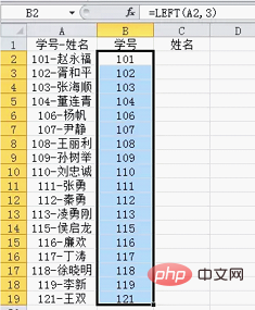
The formula is also very simple. The first parameter is the cell to extract the number, and the second parameter is the number of digits to be extracted (from Counting from the left). For this type of data in Example 1, just modify the second parameter according to the length of the number when using it.
Example 2: The numbers are on the left, the number of digits is not fixed, but there are obvious separators.
If the number length is not a fixed three digits, the previous method will not work, as shown below. At this time, you need to find the rules of the data source and then use the rules to operate. The current data uniformly has a "-" sign. You can determine the length of the number based on the position of the "-" sign, and then use left to extract it.
In this case, another function needs to be used to help, that is the find function.
Use the formula =FIND("-",A2,1) to determine the position of "-".

The find function has three parameters. The first parameter is what content to find, the second parameter is where to find it, and the third parameter is from which word Start looking (counting from the left).
=FIND("-",A2,1) means to find "-" in cell A2, starting from the beginning (the first one on the left). The result of the formula is a number, which represents the position of "-" in the cell (which character). At this time, the length of the number we need to extract is the result of find minus 1, so the method is: =LEFT(A2 ,FIND("-",A2,1)-1)

This method has a wide range of applications, as long as more obvious delimiters can be found ( It can be symbols, Chinese characters, letters, etc.), you can use this method.
Example 3:The numbers are on the left, the number of digits is not fixed and there are no obvious separators.

If the data is like this, then the previous methods cannot be used. The length of the numbers is uncertain and there are no separators. The only rule is that the data only contains numbers and Chinese characters (without letters and other symbols).
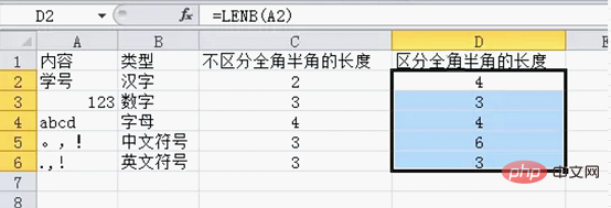
In Excel, there are two types of character lengths. Half-width characters (numbers, letters and symbols entered in English mode) have a length of 1, while full-width characters (Chinese characters and Chinese symbols, etc.) have a length of 2. You can understand this through an example:

The len function is a function that specifically calculates the length of the cell content. It does not distinguish between full-width and half-width, and its length is consistent with our usual understanding. , equivalent to the "number" of characters. Let's take a look at the difference between full-width and half-width:

The lenb function works the same as the len function. The difference is that when calculating the length of the content, half-width and full-width are distinguished. From the results, you can See a clear difference. The length of the text based on full-width is twice that of full-width and half-width, while numbers and letters are exactly the same in the two cases.
For the case of Example 3, you need to use len and lenb to determine the length of the number, and then use left to extract it.
Use the formula =LEN(A2)*2-LENB(A2) to determine the length of the number, as shown in the figure below.
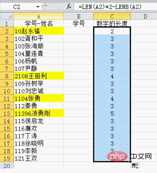
Why does len*2-lenb get the length of the number?
According to the comparison results in the previous two cases, the lenb statistical length, the text length is twice the len statistical value, and the number length is consistent with the len statistical value, so the formula len*2-lenb can be calculated The length of the number.
After counting the length of the numbers, the solution is obvious: =LEFT(A2,LEN(A2)*2-LENB(A2))
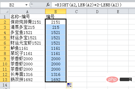
This situation in Example 3 is also typical. Just remember that it is len*2-lenb. If you really can’t remember it, you can calculate it separately when you encounter problems. First, calculate the length of the number. Just calculate it and combine left.
Example 4: The numbers are on the left and contain half-width characters such as letters.

This situation is very complicated, the only rule is that the number is on the left. Let’s see how to solve it.
You can use the formula: =-LOOKUP(1,-LEFT(A2,ROW($1:$9))).

Regarding this formula, it would probably take 5,000 words to explain, so you just need to remember the routine. The only thing that can be modified is the 9 at the end. When the longest number exceeds 9 digits, the 9 must be modified. This can be done directly with 99.
Finally, this formula works for any situation where the number is on the left .
The second type of situation: the number is on the right
The situation where the number is on the right is very similar to the number on the left. The following is only a brief explanation:
If the number of digits is fixed, use right to extract directly;

If the number of digits is not fixed but there is a delimiter, use the find function and the mid function to complete the extraction: =MID(A2,FIND("-",A2,1) 1,9)

(Note: formula The last parameter value "9" needs to be modified according to the maximum number of digits. For example, if the maximum number of digits extracted is 10, it needs to be written as 10 or a number greater than 10.)
The number of digits is not fixed at the same time If there is no delimiter, you can still use the combination of len and lenb: =RIGHT(A2,LEN(A2)*2-LENB(A2))

Continue to let lookup use big moves without any rules: =-LOOKUP(1,-RIGHT(A2,ROW($1:$9)))
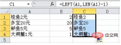
The third type of situation: the number is in the middle
The number is in the middle. This is very special. This situation generally does not occur in more standardized data sources. , let’s give an example:

For example, in the data in the picture, if the length before or after the number is fixed, you can first use a function to change the content into the situation discussed earlier. Let’s deal with it again:

#The formula is relatively simple, so I won’t explain it. As for how to do the next step, you already know it based on the previous studies, right?
The method I will talk about below is a more general method. Some people call it the universal extraction formula:
=-LOOKUP(0,-MID(A1,MIN (FIND(ROW($1:$10)-1,A1&1/17)),ROW($1:$9)))

Ctrl shift Enter" to end.
Summary
Regarding how to use formulas to extract numbers in cells, the above has explained most of the situations, but of course not all , for example, when it contains decimals, it is even more special because of the decimal point.The last array formula can be regarded as a more general formula. What needs to be emphasized is that most problems become very troublesome because of non-standard data sources. Therefore, develop a good habit of storing only one attribute of data in a cell, such as name and quantity, Price and other information are stored separately, which will greatly improve statistical efficiency.
Of course, from the perspective of improving the ability to use formulas, problems such as number extraction are also good topics for function practice. I hope you can combine the functions you have learned before and think of more formulas to extract numbers.
Related learning recommendations: excel tutorial
The above is the detailed content of Practical Excel skills sharing: How to extract numbers?. For more information, please follow other related articles on the PHP Chinese website!

Hot AI Tools

Undresser.AI Undress
AI-powered app for creating realistic nude photos

AI Clothes Remover
Online AI tool for removing clothes from photos.

Undress AI Tool
Undress images for free

Clothoff.io
AI clothes remover

AI Hentai Generator
Generate AI Hentai for free.

Hot Article

Hot Tools

Notepad++7.3.1
Easy-to-use and free code editor

SublimeText3 Chinese version
Chinese version, very easy to use

Zend Studio 13.0.1
Powerful PHP integrated development environment

Dreamweaver CS6
Visual web development tools

SublimeText3 Mac version
God-level code editing software (SublimeText3)

Hot Topics
 1385
1385
 52
52
 What should I do if the frame line disappears when printing in Excel?
Mar 21, 2024 am 09:50 AM
If when opening a file that needs to be printed, we will find that the table frame line has disappeared for some reason in the print preview. When encountering such a situation, we must deal with it in time. If this also appears in your print file If you have questions like this, then join the editor to learn the following course: What should I do if the frame line disappears when printing a table in Excel? 1. Open a file that needs to be printed, as shown in the figure below. 2. Select all required content areas, as shown in the figure below. 3. Right-click the mouse and select the "Format Cells" option, as shown in the figure below. 4. Click the “Border” option at the top of the window, as shown in the figure below. 5. Select the thin solid line pattern in the line style on the left, as shown in the figure below. 6. Select "Outer Border"
 How to filter more than 3 keywords at the same time in excel
Mar 21, 2024 pm 03:16 PM
Excel is often used to process data in daily office work, and it is often necessary to use the "filter" function. When we choose to perform "filtering" in Excel, we can only filter up to two conditions for the same column. So, do you know how to filter more than 3 keywords at the same time in Excel? Next, let me demonstrate it to you. The first method is to gradually add the conditions to the filter. If you want to filter out three qualifying details at the same time, you first need to filter out one of them step by step. At the beginning, you can first filter out employees with the surname "Wang" based on the conditions. Then click [OK], and then check [Add current selection to filter] in the filter results. The steps are as follows. Similarly, perform filtering separately again
 How to change excel table compatibility mode to normal mode
Mar 20, 2024 pm 08:01 PM
In our daily work and study, we copy Excel files from others, open them to add content or re-edit them, and then save them. Sometimes a compatibility check dialog box will appear, which is very troublesome. I don’t know Excel software. , can it be changed to normal mode? So below, the editor will bring you detailed steps to solve this problem, let us learn together. Finally, be sure to remember to save it. 1. Open a worksheet and display an additional compatibility mode in the name of the worksheet, as shown in the figure. 2. In this worksheet, after modifying the content and saving it, the dialog box of the compatibility checker always pops up. It is very troublesome to see this page, as shown in the figure. 3. Click the Office button, click Save As, and then
 How to type subscript in excel
Mar 20, 2024 am 11:31 AM
eWe often use Excel to make some data tables and the like. Sometimes when entering parameter values, we need to superscript or subscript a certain number. For example, mathematical formulas are often used. So how do you type the subscript in Excel? ?Let’s take a look at the detailed steps: 1. Superscript method: 1. First, enter a3 (3 is superscript) in Excel. 2. Select the number "3", right-click and select "Format Cells". 3. Click "Superscript" and then "OK". 4. Look, the effect is like this. 2. Subscript method: 1. Similar to the superscript setting method, enter "ln310" (3 is the subscript) in the cell, select the number "3", right-click and select "Format Cells". 2. Check "Subscript" and click "OK"
 How to set superscript in excel
Mar 20, 2024 pm 04:30 PM
When processing data, sometimes we encounter data that contains various symbols such as multiples, temperatures, etc. Do you know how to set superscripts in Excel? When we use Excel to process data, if we do not set superscripts, it will make it more troublesome to enter a lot of our data. Today, the editor will bring you the specific setting method of excel superscript. 1. First, let us open the Microsoft Office Excel document on the desktop and select the text that needs to be modified into superscript, as shown in the figure. 2. Then, right-click and select the "Format Cells" option in the menu that appears after clicking, as shown in the figure. 3. Next, in the “Format Cells” dialog box that pops up automatically
 How to use the iif function in excel
Mar 20, 2024 pm 06:10 PM
Most users use Excel to process table data. In fact, Excel also has a VBA program. Apart from experts, not many users have used this function. The iif function is often used when writing in VBA. It is actually the same as if The functions of the functions are similar. Let me introduce to you the usage of the iif function. There are iif functions in SQL statements and VBA code in Excel. The iif function is similar to the IF function in the excel worksheet. It performs true and false value judgment and returns different results based on the logically calculated true and false values. IF function usage is (condition, yes, no). IF statement and IIF function in VBA. The former IF statement is a control statement that can execute different statements according to conditions. The latter
 Where to set excel reading mode
Mar 21, 2024 am 08:40 AM
In the study of software, we are accustomed to using excel, not only because it is convenient, but also because it can meet a variety of formats needed in actual work, and excel is very flexible to use, and there is a mode that is convenient for reading. Today I brought For everyone: where to set the excel reading mode. 1. Turn on the computer, then open the Excel application and find the target data. 2. There are two ways to set the reading mode in Excel. The first one: In Excel, there are a large number of convenient processing methods distributed in the Excel layout. In the lower right corner of Excel, there is a shortcut to set the reading mode. Find the pattern of the cross mark and click it to enter the reading mode. There is a small three-dimensional mark on the right side of the cross mark.
 How to insert excel icons into PPT slides
Mar 26, 2024 pm 05:40 PM
1. Open the PPT and turn the page to the page where you need to insert the excel icon. Click the Insert tab. 2. Click [Object]. 3. The following dialog box will pop up. 4. Click [Create from file] and click [Browse]. 5. Select the excel table to be inserted. 6. Click OK and the following page will pop up. 7. Check [Show as icon]. 8. Click OK.


