

Practical Excel skills sharing: 'Data Validity' can be used in this way!

In the previous article " Practical Excel skills sharing: How to extract numbers? ", we explain several common types of data extraction situations. Today we are going to talk about Excel’s “data validity” function and share 3 tips to make data validity more efficient. Come and learn!
Everyone should use the "data validity" function quite a lot in their work, right? Most people commonly use it for selection drop-downs, data entry restrictions, etc. Today Bottle will introduce to you some functions that may seem inconspicuous but are actually very efficient and warm.
1. Make a drop-down list with "Super Table"
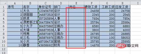
For the table as shown below, you need to make a drop-down list in column E. This way you don't have to manually enter the position, you can select it directly from the drop-down list.
At this time, most people may click on the data validity dialog box and directly enter the required content in the drop-down list manually.

#There is a drawback to this. When a new position is added, the data validity needs to be reset. We can create a dedicated table as a source here. Create a basic information table in the workbook. As shown in the figure below, name Table 2 as the basic information table.
Click "Insert" - "Table" in cell A1 of the basic information table.
#The "Create Table" dialog box pops up, click "OK" directly to see the super table in the table.
Directly enter the company’s existing positions in the form, and the super table will automatically expand, as shown below.
Select the entire data area, set a name for this column of data in the name box above the table, such as "Position", and press Enter to confirm.
After setting the name, click "Formula" - "Use for formula". You can see the name we just customized in the drop-down menu, which can be called at any time. This will also be used in future function learning.
Go back to the original salary table, select the data in column E, and click "Data" - "Data Validity".

In the pop-up dialog box, select "Sequence" in the "Allow" drop-down menu.

Click in the input box below "Source", and then click the "Formula" tab "Used for Formulas" - "Position". At this point you can see that the "Position" table area is called in "Source".

After clicking "OK", a drop-down button will appear after the data in column E. Click the button to select a position in the drop-down list.
#If there are new positions at this time, add content directly to the "Position" super table in the basic information table. As shown in the picture below, I entered the newly added position of R&D Director in cell A12.
#After pressing Enter, you can see that the table is automatically expanded and the new positions are included in the "Positions" table area.
At this point we return to the salary table and look at the drop-down list of any cell in column E. We can see that "R&D Director" has been added to the end of the list.
For those who use the excel2010 version, please note that after using the super table, the data validity may be "invalid". In this case, you only need to uncheck "Ignore null values". .

2. Humanized warning message
In the table as shown below, select column C Data, formatted as text. Because our ID numbers are all 18-digit long numbers and will not participate in mathematical operations, we can set the entire column in text format in advance.
Call up the data validity dialog box and enter the text length - equal to -18.
When you enter a string of numbers without 18 digits in cell C2, a warning message will pop up as shown in the figure below.
The warning message at this time looks very stiff, and it is possible that people using the form cannot understand it. We can customize a humanized warning message to let people know how to do it. operate.
After selecting the data in the ID card column, bring up the data validity dialog box and click the "Error Warning" tab. We can see the dialog box shown below.
Click the "Style" drop-down list, there are three methods: "Stop", "Warning" and "Information". "Stop" means that when the user enters incorrect information, the information cannot be entered into the cell. "Warning" means that when the user enters incorrect information, the user is reminded. After the user clicks OK again, the information can be entered into the cell. "Information" means that when the user enters incorrect information, it only reminds the user that the information has been entered into the cell.
#On the right side of the dialog box, we can set the title and prompt content of the warning message, as shown below.
After clicking OK, when the number entered in cell C2 is not 18 digits, a prompt box for our custom settings will pop up.
3. Circle the error data and empty cells
As shown below, when I After setting column C as "warning" information, the user entered incorrect data and clicked OK again, but it was still saved. At this time I need to mark out the incorrect data.
Select the data in column C and click "Data" - "Data Validity" - "Circle Invalid Data".
At this time, the incorrect data entered in the ID card column will be marked. However, the empty cells with no information entered are not marked.
If you want to circle the empty cells with no entered information, we click "Clear Invalid Data Identification Circles" in the "Data Validity" drop-down list to clear it first. Logo circle.

Then select the data area, bring up the data validity dialog box, and uncheck "Ignore null values" in the "Settings" dialog box.

At this time, perform the previous circle release operation, and you can see that the cells with entered error information and empty cells have been circled and released.

#When our company has hundreds of people, we can easily find the missed cells using this method.
That’s it for today’s tutorial, have you learned it? Making good use of data validity can save a lot of time when statistics are collected.
Related learning recommendations: excel tutorial
The above is the detailed content of Practical Excel skills sharing: 'Data Validity' can be used in this way!. For more information, please follow other related articles on the PHP Chinese website!

Hot AI Tools

Undresser.AI Undress
AI-powered app for creating realistic nude photos

AI Clothes Remover
Online AI tool for removing clothes from photos.

Undress AI Tool
Undress images for free

Clothoff.io
AI clothes remover

AI Hentai Generator
Generate AI Hentai for free.

Hot Article
Hot Tools

Notepad++7.3.1
Easy-to-use and free code editor

SublimeText3 Chinese version
Chinese version, very easy to use

Zend Studio 13.0.1
Powerful PHP integrated development environment

Dreamweaver CS6
Visual web development tools

SublimeText3 Mac version
God-level code editing software (SublimeText3)
Hot Topics
 1378
1378
 52
52

 What should I do if the frame line disappears when printing in Excel?
Mar 21, 2024 am 09:50 AM
What should I do if the frame line disappears when printing in Excel?
Mar 21, 2024 am 09:50 AM
If when opening a file that needs to be printed, we will find that the table frame line has disappeared for some reason in the print preview. When encountering such a situation, we must deal with it in time. If this also appears in your print file If you have questions like this, then join the editor to learn the following course: What should I do if the frame line disappears when printing a table in Excel? 1. Open a file that needs to be printed, as shown in the figure below. 2. Select all required content areas, as shown in the figure below. 3. Right-click the mouse and select the "Format Cells" option, as shown in the figure below. 4. Click the “Border” option at the top of the window, as shown in the figure below. 5. Select the thin solid line pattern in the line style on the left, as shown in the figure below. 6. Select "Outer Border"
 How to filter more than 3 keywords at the same time in excel
Mar 21, 2024 pm 03:16 PM
How to filter more than 3 keywords at the same time in excel
Mar 21, 2024 pm 03:16 PM
Excel is often used to process data in daily office work, and it is often necessary to use the "filter" function. When we choose to perform "filtering" in Excel, we can only filter up to two conditions for the same column. So, do you know how to filter more than 3 keywords at the same time in Excel? Next, let me demonstrate it to you. The first method is to gradually add the conditions to the filter. If you want to filter out three qualifying details at the same time, you first need to filter out one of them step by step. At the beginning, you can first filter out employees with the surname "Wang" based on the conditions. Then click [OK], and then check [Add current selection to filter] in the filter results. The steps are as follows. Similarly, perform filtering separately again
 How to change excel table compatibility mode to normal mode
Mar 20, 2024 pm 08:01 PM
How to change excel table compatibility mode to normal mode
Mar 20, 2024 pm 08:01 PM
In our daily work and study, we copy Excel files from others, open them to add content or re-edit them, and then save them. Sometimes a compatibility check dialog box will appear, which is very troublesome. I don’t know Excel software. , can it be changed to normal mode? So below, the editor will bring you detailed steps to solve this problem, let us learn together. Finally, be sure to remember to save it. 1. Open a worksheet and display an additional compatibility mode in the name of the worksheet, as shown in the figure. 2. In this worksheet, after modifying the content and saving it, the dialog box of the compatibility checker always pops up. It is very troublesome to see this page, as shown in the figure. 3. Click the Office button, click Save As, and then
 How to type subscript in excel
Mar 20, 2024 am 11:31 AM
How to type subscript in excel
Mar 20, 2024 am 11:31 AM
eWe often use Excel to make some data tables and the like. Sometimes when entering parameter values, we need to superscript or subscript a certain number. For example, mathematical formulas are often used. So how do you type the subscript in Excel? ?Let’s take a look at the detailed steps: 1. Superscript method: 1. First, enter a3 (3 is superscript) in Excel. 2. Select the number "3", right-click and select "Format Cells". 3. Click "Superscript" and then "OK". 4. Look, the effect is like this. 2. Subscript method: 1. Similar to the superscript setting method, enter "ln310" (3 is the subscript) in the cell, select the number "3", right-click and select "Format Cells". 2. Check "Subscript" and click "OK"
 How to set superscript in excel
Mar 20, 2024 pm 04:30 PM
How to set superscript in excel
Mar 20, 2024 pm 04:30 PM
When processing data, sometimes we encounter data that contains various symbols such as multiples, temperatures, etc. Do you know how to set superscripts in Excel? When we use Excel to process data, if we do not set superscripts, it will make it more troublesome to enter a lot of our data. Today, the editor will bring you the specific setting method of excel superscript. 1. First, let us open the Microsoft Office Excel document on the desktop and select the text that needs to be modified into superscript, as shown in the figure. 2. Then, right-click and select the "Format Cells" option in the menu that appears after clicking, as shown in the figure. 3. Next, in the “Format Cells” dialog box that pops up automatically
 How to use the iif function in excel
Mar 20, 2024 pm 06:10 PM
How to use the iif function in excel
Mar 20, 2024 pm 06:10 PM
Most users use Excel to process table data. In fact, Excel also has a VBA program. Apart from experts, not many users have used this function. The iif function is often used when writing in VBA. It is actually the same as if The functions of the functions are similar. Let me introduce to you the usage of the iif function. There are iif functions in SQL statements and VBA code in Excel. The iif function is similar to the IF function in the excel worksheet. It performs true and false value judgment and returns different results based on the logically calculated true and false values. IF function usage is (condition, yes, no). IF statement and IIF function in VBA. The former IF statement is a control statement that can execute different statements according to conditions. The latter
 Where to set excel reading mode
Mar 21, 2024 am 08:40 AM
Where to set excel reading mode
Mar 21, 2024 am 08:40 AM
In the study of software, we are accustomed to using excel, not only because it is convenient, but also because it can meet a variety of formats needed in actual work, and excel is very flexible to use, and there is a mode that is convenient for reading. Today I brought For everyone: where to set the excel reading mode. 1. Turn on the computer, then open the Excel application and find the target data. 2. There are two ways to set the reading mode in Excel. The first one: In Excel, there are a large number of convenient processing methods distributed in the Excel layout. In the lower right corner of Excel, there is a shortcut to set the reading mode. Find the pattern of the cross mark and click it to enter the reading mode. There is a small three-dimensional mark on the right side of the cross mark.
 How to insert excel icons into PPT slides
Mar 26, 2024 pm 05:40 PM
How to insert excel icons into PPT slides
Mar 26, 2024 pm 05:40 PM
1. Open the PPT and turn the page to the page where you need to insert the excel icon. Click the Insert tab. 2. Click [Object]. 3. The following dialog box will pop up. 4. Click [Create from file] and click [Browse]. 5. Select the excel table to be inserted. 6. Click OK and the following page will pop up. 7. Check [Show as icon]. 8. Click OK.
